On March 22, 2018 we renamed the Awesome Plan to the Pro Plan, and changed its price from $10/mo to $15/mo. We announced the change and offered a promotion to let users lock in the $10/mo. price one month earlier, on February 22.
In this analysis we’ll analyze the effect that the price change has had on mobile revenue. In our previous analyses we’ve focused only on Stripe revenue and overlooked mobile. This analysis is at least 6 months late, but better late than never.
We’ll utilize the Causal Impact package to estimate what MRR would have been without the price change and calculate the effect size from there. It’s important to note that the effect of the annual plan promotion likely interacts with the effect of the price change, so any effect on MRR will have come as a result of both events.
Summary
We may have underestimated the impact that the price change would have on mobile revenue. The impact on mobile is very different than that on web-based revenue. Perhaps people are more sensitive to price differences when paying for something in the mobile app stores. The cumulative effect of the price changes on mobile revenue seems to be somewhere around a $25K loss in MRR.
We’ll collect mobile MRR data for all dates since June 2017.
select
  date(date) as date
  , plan_id
  , gateway
  , billing_cycle
  , total_mrr
from dbt.daily_mrr_values
where gateway in ('Apple', 'Android')
and date >= '2017-06-01'
Now that we’ve collected the data, let’s plot mobile MRR over the course of 2018.
## `summarise()` regrouping output by 'date' (override with `.groups` argument)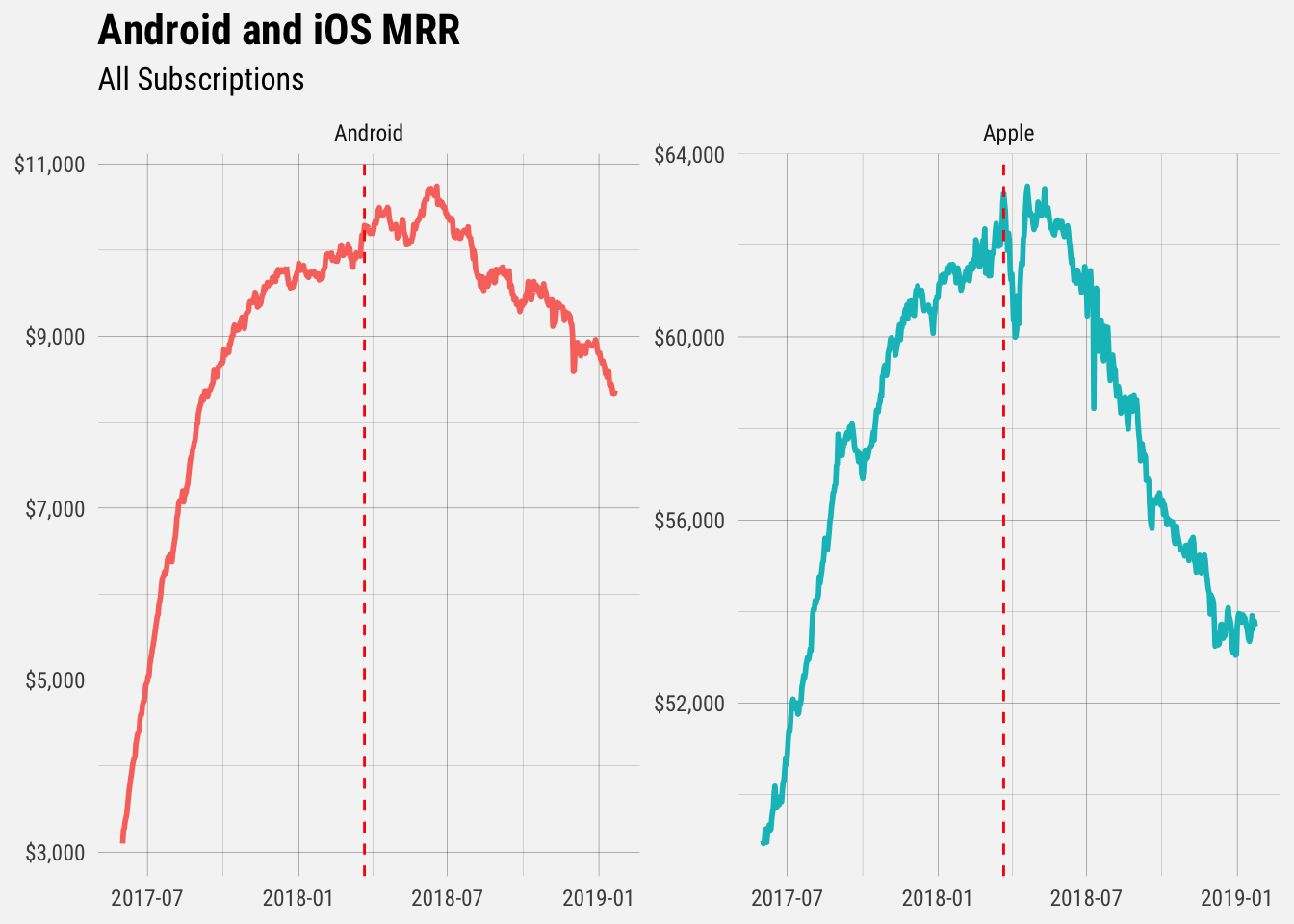
Oh dear. The red dotted line represents the date that the price change fully went into effect. Although revenue growth had already slowed for both Android and Apple, the date of the price change seems to conincide with a peak in mobile revenue, followed by a marked decline.
If we look only at monthly subscriptions, we can see the effect more clearly.
## `summarise()` regrouping output by 'date' (override with `.groups` argument)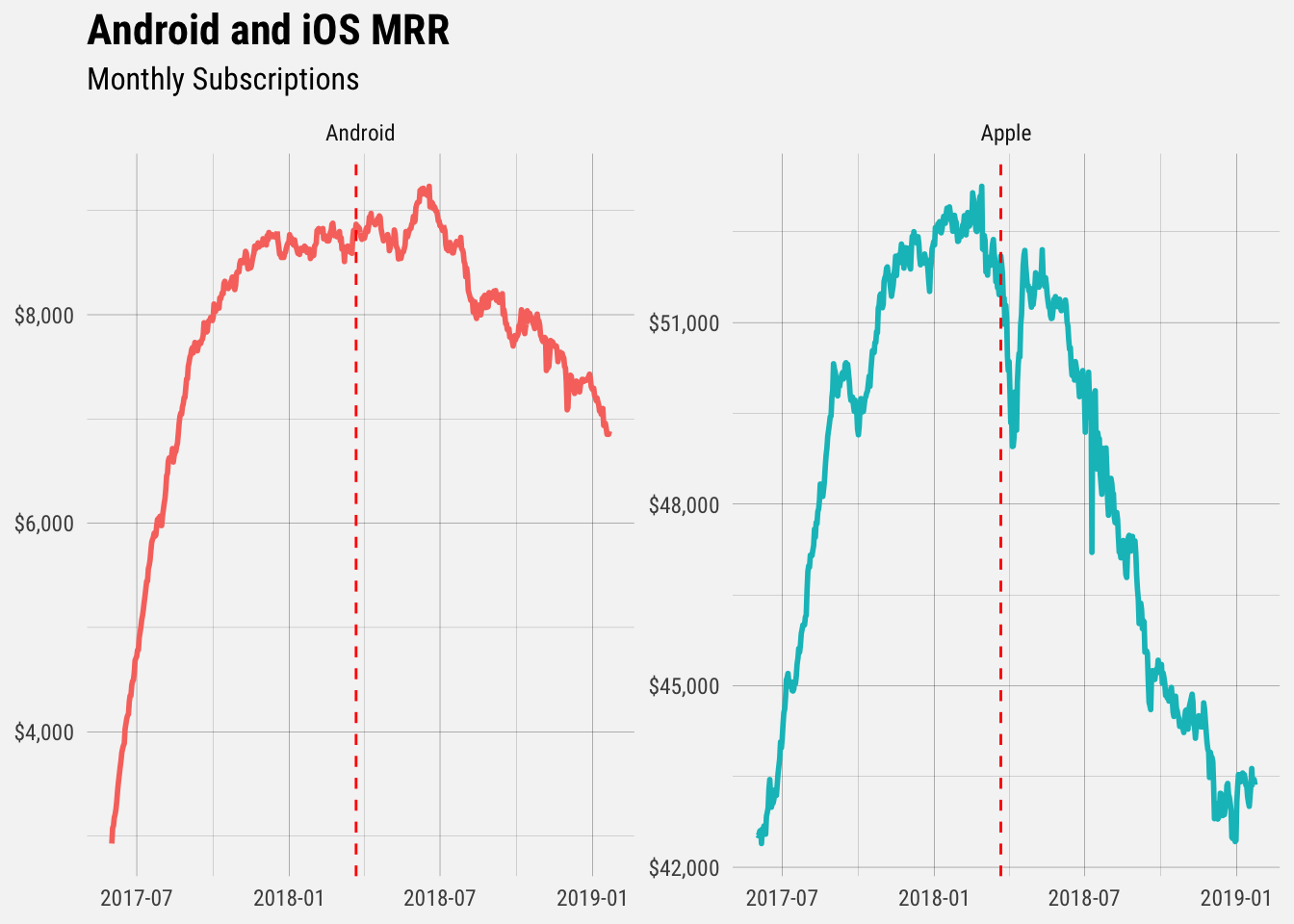
Measuring the Effect on MRR
We’ll use a technique called Causal Impact for causal inference. Essentially, we take MRR growth before the pricing change and forecast it into the future, and compare the forecast with the observed values. The difference between the counterfactual (what MRR growth would have happened without the pricing change) and the observed MRR growth numbers is our estimated effect size.
We’ll also try to isolate the effect of the price change by excluding the weeks during which the promotional offer had a large effect. We do this by defining the “post-intervention period” as the weeks from April 2 onwards.
The “pre-intervention period”" includes dates from June 1, 2017 to the week of February 26, which is the week that we announced the price change and the offer to lock in the lower prices. We use the average MRR growth from the dates in the pre-intervention period to create our forecast of what MRR growth would have looked like without the pricing change. In this case, the simple average of is used.
You’ll notice that we’ve left out a few weeks in March. The weeks of March 19 and March 26 saw unusually high MRR growth, and it’s my assumption is that this was primarily due to our offer to let users lock in the lower prices. We’ll use the weeks outside of this time window for our analysis.
To perform inference, we run the analysis using the CausalImpact command.
# run analysis
impact <- CausalImpact(mrr_ts, pre.period, post.period, model.args = list(niter = 5000))

# plot impact
plot(impact) +
  labs(title = "Impact on Mobile MRR", subtitle = "Estimated Cumulative Loss of $20K in MRR") +
  scale_y_continuous(labels = dollar) +
  buffer_theme()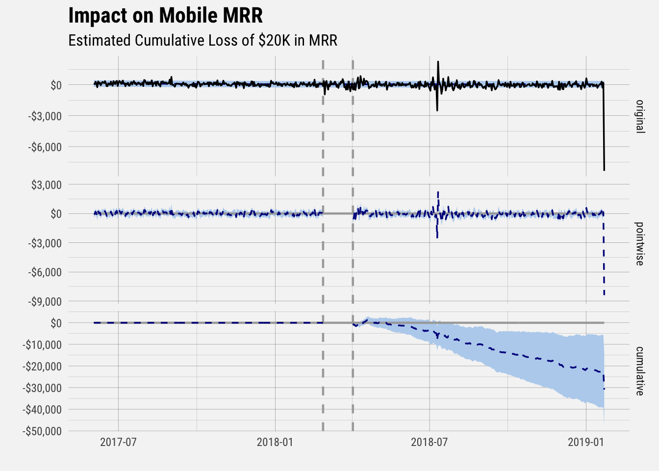
The pre-intervention period includes all data to the left of the first vertical dotted line, and the post-intervention period includes all data to the right of the second vertical dotted line.
The top panel in the graph shows the actual observed data (the black line) as well as the counterfactual, which is our best guess at what daily MRR growth would have been had we not introduced a new plan.
The second panel displays the estimated effect that the price change had on MRR growth each day, and the bottom panel shows the cumulative effect over time on daily MRR growth.
Because there are so many points, it’s difficult to see the pointwise estimates, i.e. the the estimated change in daily MRR growth for each day. The cumulative effect of these daily changes in MRR growth can be clearly seen in the bottom panel however. The cumulative effect appears to be somewhere around a $25 thousand loss in MRR.
Lets’s look at the summary of our causal impact model.
# get summary
summary(impact)
## Posterior inference {CausalImpact}
##
## Average Cumulative
## Actual -60 -17770
## Prediction (s.d.) 44 (29) 13143 (8717)
## 95% CI [-13, 101] [-3936, 29873]
##
## Absolute effect (s.d.) -104 (29) -30913 (8717)
## 95% CI [-161, -47] [-47643, -13833]
##
## Relative effect (s.d.) -235% (66%) -235% (66%)
## 95% CI [-362%, -105%] [-362%, -105%]
##
## Posterior tail-area probability p: 4e-04
## Posterior prob. of a causal effect: 99.95977%
##
## For more details, type: summary(impact, "report")The probability of a true causal effect is well over 99%. Average daily MRR growth for the mobile apps was $44 per day before February 26, and -$60 per day for the dates following March 26. This equates a relative effect of around -238%.