We’re currently working with Twitter to finalize our contract for the next 12 months and there is a possibility to lock in the next pricing tier for the API that Reply uses. In order to make an informed decision on this, we would like to forecast the number of Twitter handles used in Reply. We currently pay $11,250/mo for 1,000 Twitter handles.
Data Collection
The Reply data we need lives in BigQuery. We can collect this data with the bigrquery package.
# load DBI package
library(DBI)

# connect to BigQuery
con <- dbConnect(
  bigrquery::bigquery(),
  project = "buffer-data",
  dataset = "atlas_reply_meteor"
)
Let’s start by querying the twitter_accounts table.
# define sql query
sql <- "
  select
    _id as id
    , created_at
    , name
  from twitter_accounts
"

# collect data
profiles <- dbGetQuery(con, sql)
There are 26 thousand Twitter profiles in this dataset. Not all of them are currently being used though.
Let’s quickly plot the cumulative sum of the number of Twitter profiles connected to Reply across all time.
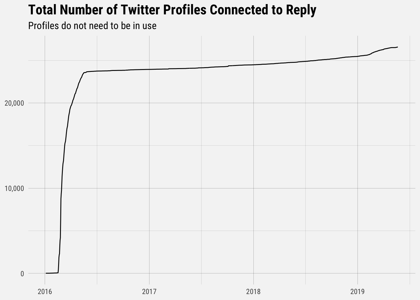
We can see that the number of Twitter profiles really ramped up in early 2016, and has increased slowly since then. What we need, though, is to see the number of Twitter profiles being used.
Twitter Conversations
We will use the conversations table to get a better sense of how many Twitter profiles are in use.
# define sql query
sql <- "
  select
    _id as id
    , timestamp_millis(cast(created_at as INT64)) as created_at
    , contact_ref
    , source
  from conversations
  where type = 'twitter'
  and timestamp_millis(cast(created_at as INT64)) >= '2018-01-01'
"

# collect data
conversations <- dbGetQuery(con, sql)
There are 7.8 million Twitter conversations in this dataset. Let’s extract the profile ids.
# extract the twitter profile id
conversations <- conversations %>%
  mutate(profile_id = str_sub(source, start = 7, end = 22))
Now let’s group the data by month and count the profile ids.
# group by month
by_month <- conversations %>%
  mutate(month = floor_date(created_at, unit = "months")) %>%
  group_by(month) %>%
  summarise(profiles = n_distinct(profile_id))
## `summarise()` ungrouping output (override with `.groups` argument)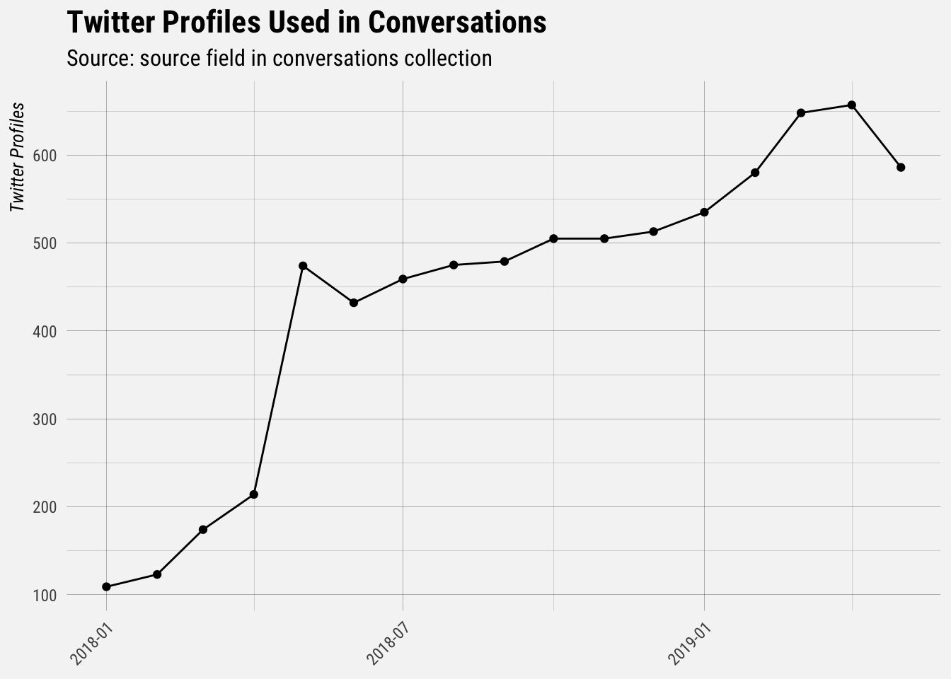
It looks like there was a big spike in May 2018. Let’s only look at data beyond that point, so that we have less noise when making our predictions.
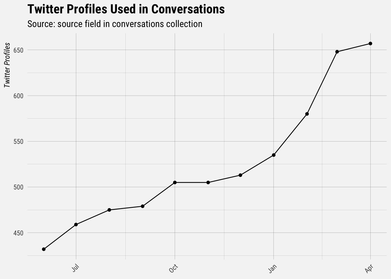
Great, we can use this dataset to make our forecasts.
Forecasting Twitter Usage
We’ll use the prophet package developed by the folks at Facebook to make our basic forecasts. We first need to prep a dataframe with columns ds and y, containing the date and numeric value respectively. The ds column should be YYYY-MM-DD for a date, or YYYY-MM-DD HH:MM:SS for a timestamp.
# create dataframe to send to prophet
prophet_df <- by_month %>%
  filter(month > "2018-05-01" & month < "2019-04-02") %>%
  rename(ds = month, y = profiles)

# fit model
mod <- prophet(prophet_df, algorithm = 'LBFGS')
Predictions are made on a dataframe with a column ds containing the dates for which predictions are to be made. The make_future_dataframe function takes the model object and a number of periods to forecast and produces a suitable dataframe. By default it will also include the historical dates so we can evaluate in-sample fit.
# make future dataframe
future <- make_future_dataframe(mod, periods = 24, freq = "month")

# view dataframe
tail(future)
## ds
## 30 2020-11-01
## 31 2020-12-01
## 32 2021-01-01
## 33 2021-02-01
## 34 2021-03-01
## 35 2021-04-01Now let’s make the forecast and plot the results.
# make predictions
fcast <- predict(mod, future)

# plot results
plot(mod, fcast) +
  geom_point(data = filter(fcast, ds > "2019-04-01"), aes(x = ds, y = yhat), color = "red") +
  buffer_theme() +
  labs(x = "Month",
       y = "Twitter Profiles",
       title = "Forecasted Monthly Twitter Profile Usage",
       subtitle = "Based on conversations data from June 2018")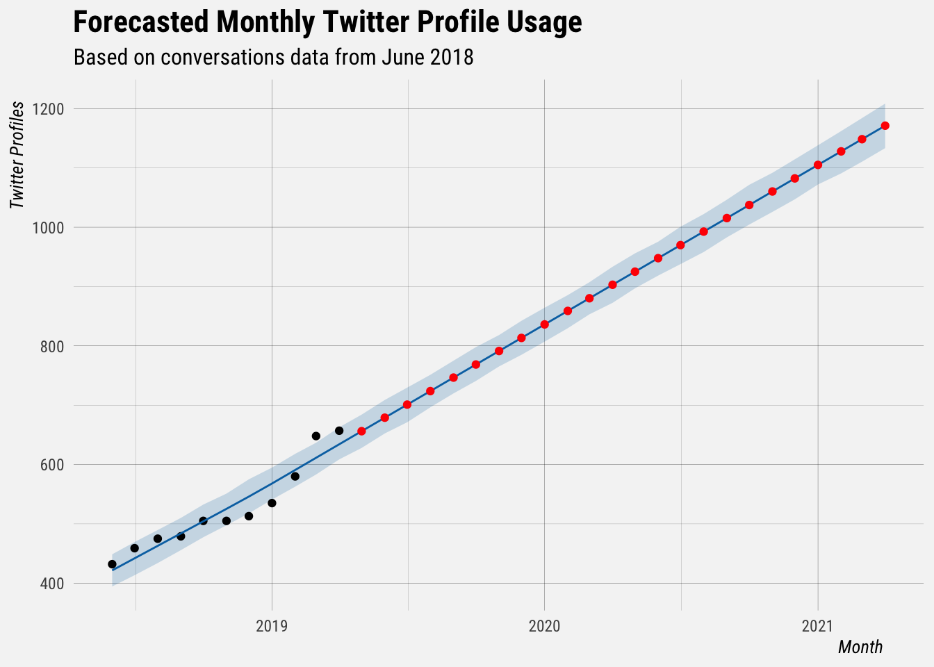
The red dots are the forecasted values. This forecast assumes a linear growth trend. The biggest source of uncertainty in the forecast is the potential for future trend changes, so the furthest months forecasted for have the highest risk of being off.
Let’s get the forecasted values and the confidence intervals. The upper_bound and lower_bound represent the uncertainty interval, which is based on the variance between historic months. You can see that most of the black dots in the plot above fall within this uncertainty interval.
# get forecasted values
fcast %>%
  filter(ds > "2019-03-01") %>%
  rename(month = ds, forecast = yhat, lower_bound = yhat_lower, upper_bound = yhat_upper) %>%
  select(month, forecast, lower_bound, upper_bound) %>%
  kable() %>%
kable_styling()| month | forecast | lower_bound | upper_bound |
|---|---|---|---|
| 2019-04-01 | 634.1375 | 608.6299 | 662.7920 |
| 2019-05-01 | 656.1768 | 627.9576 | 684.1446 |
| 2019-06-01 | 678.9506 | 652.3466 | 708.8711 |
| 2019-07-01 | 700.9899 | 671.2298 | 729.6538 |
| 2019-08-01 | 723.7637 | 696.4023 | 751.2596 |
| 2019-09-01 | 746.5376 | 719.8588 | 775.0730 |
| 2019-10-01 | 768.5768 | 740.8721 | 797.9336 |
| 2019-11-01 | 791.3507 | 765.3178 | 818.2959 |
| 2019-12-01 | 813.3899 | 784.9486 | 842.2773 |
| 2020-01-01 | 836.1638 | 807.1164 | 864.3463 |
| 2020-02-01 | 858.9376 | 829.7618 | 885.6040 |
| 2020-03-01 | 880.2422 | 853.1739 | 907.3562 |
| 2020-04-01 | 903.0161 | 872.5290 | 933.3749 |
| 2020-05-01 | 925.0553 | 896.9510 | 955.9541 |
| 2020-06-01 | 947.8292 | 918.4374 | 975.5849 |
| 2020-07-01 | 969.8684 | 937.8465 | 1000.8841 |
| 2020-08-01 | 992.6423 | 958.1739 | 1022.1814 |
| 2020-09-01 | 1015.4161 | 982.8991 | 1046.3971 |
| 2020-10-01 | 1037.4554 | 1004.4724 | 1071.5213 |
| 2020-11-01 | 1060.2292 | 1025.7754 | 1091.7295 |
| 2020-12-01 | 1082.2685 | 1046.9983 | 1114.4758 |
| 2021-01-01 | 1105.0423 | 1072.0014 | 1138.1637 |
| 2021-02-01 | 1127.8162 | 1090.6953 | 1162.0433 |
| 2021-03-01 | 1148.3861 | 1110.4519 | 1184.0244 |
| 2021-04-01 | 1171.1600 | 1133.3345 | 1208.3989 |
Based on this linear growth, we would start getting close to hitting 1000 profiles per month around August or September of 2020.
Tracking Usage Across Social Networks
Let’s see how Twitter usage compares with usage of the other social networks. We’ll use DBI in conjunction with the bigrquery package to collect the data.
# define sql query
sql <- "
  select
    extract(month from timestamp_millis(cast(created_at as INT64))) as month
    , extract(year from timestamp_millis(cast(created_at as INT64))) as year
    , type
    , array(select * from unnest(split(substr(source, 2 , length(source) - 2))))[offset(1)] as profile_id
    , count(distinct _id) as conversations
  from atlas_reply_meteor.conversations
  where timestamp_millis(cast(created_at as INT64)) >= '2018-01-01'
  group by 1, 2, 3, 4
"

# collect data
convos <- dbGetQuery(con, sql)
# create date year column and trim whitespace
convos <- convos %>%
mutate(month = gsub(" ", "0", format(month, digits = 2)),
yearmon = paste(year, month, sep = "-"),
profile_id = trimws(profile_id, which = c("both")))Now let’s plot the growth by month.
## `summarise()` regrouping output by 'yearmon' (override with `.groups` argument)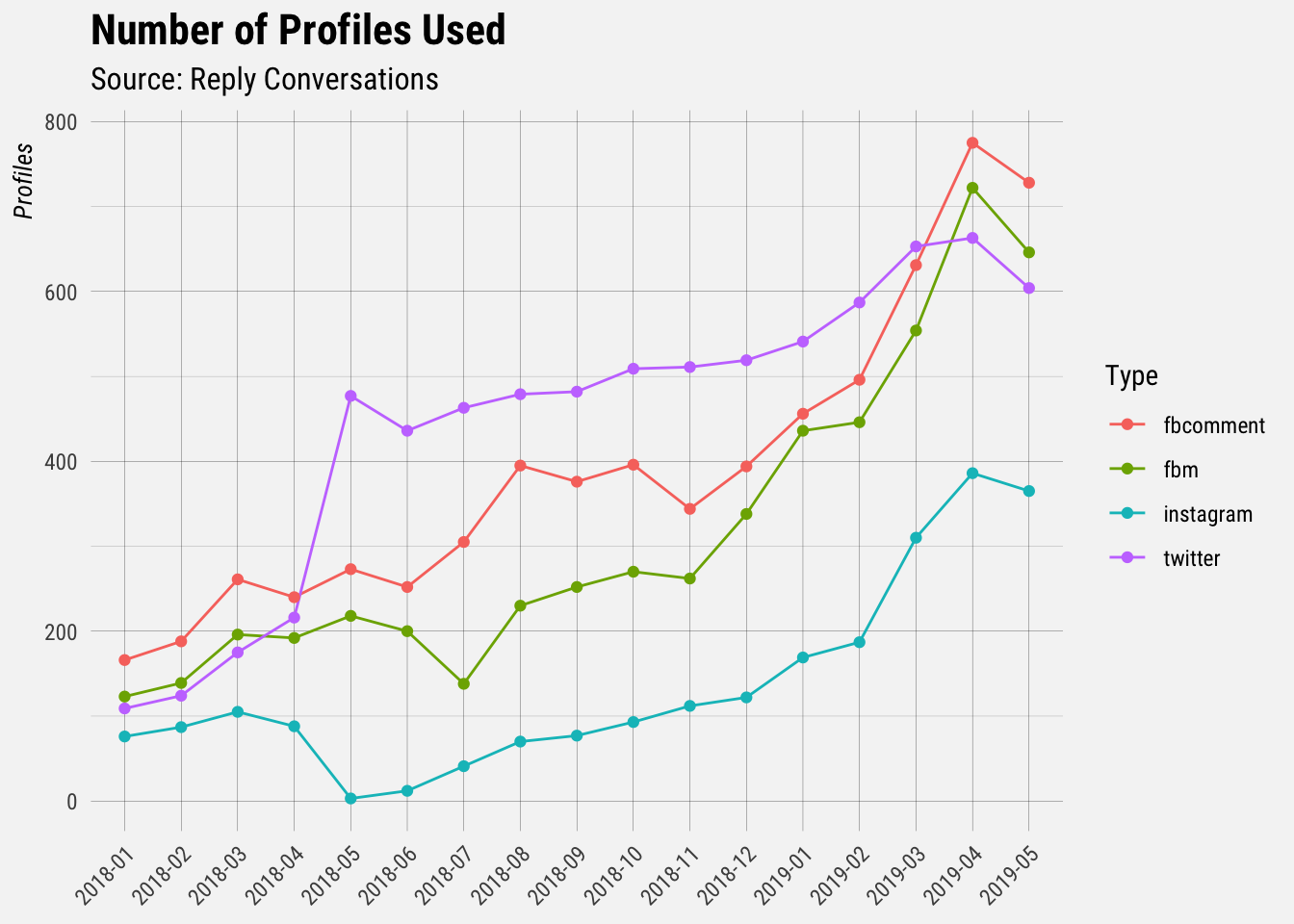
It looks like Facebook has overtaken Twitter as the most popular network in recent months!