# connect to BigQuery
con <- dbConnect(
  bigrquery::bigquery(),
  project = "buffer-data"
)

# define sql query
sql <- "
  select *
  from dbt_buffer.stripe_paid_subscriptions
  where created_at >= '2019-01-01'
  and plan_id in ('business_v2_small_monthly', 'business_v2_small_yearly',
  'premium_business_v1_monthly', 'premium_business_v1_yearly',
  'business_v2_business_monthly', 'business_v2_business_yearly',
  'business_v2_agency_monthly', 'business_v2_agency_yearly',
  'publish_premium_m_35_201910', 'publish_premium_y_336_201910')
"

# query bigquery
subs <- dbGetQuery(con, sql)

# get plan interval
subs <- subs %>%
  mutate(interval = ifelse(grepl("month", plan_id) | plan_id == "publish_premium_m_35_201910",
                           "month", "year"),
         created_date = as.Date(created_at, format = "%Y-%m-%d"),
         cancel_date = as.Date(canceled_at, format = "%Y-%m-%d"),
         canceled = !is.na(cancel_date),
         days_to_cancel = ifelse(canceled,
                                 as.numeric(cancel_date - created_date),
                                 as.numeric(Sys.Date() - created_date)))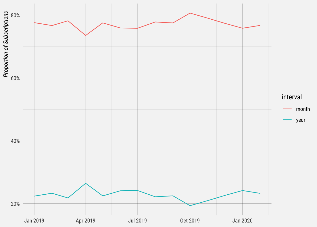
Survival Analysis
# build survival object
km <- Surv(subs$days_to_cancel, subs$canceled)

# preview data
head(km, 20)
## [1] 160+ 400+ 157+ 221 409+ 56 409+ 325 295+ 245+ 372+ 141+ 381+ 359+ 38
## [16] 61 178+ 36 14+ 266To begin our analysis, we use the formula Surv(time, canceled) ~ 1 and the survfit() function to produce the Kaplan-Meier estimates of the probability of “survival” over time. The times parameter of the summary() function gives some control over which times to print. Here, it is set to print the estimates for 1, 30, 60 and 90 days, and then every 90 days thereafter.
# get survival probabilities
km_fit <- survfit(Surv(days_to_cancel, canceled) ~ 1, data = subs)

# summarise
summary(km_fit, times = c(1, 7, 14, 30, 60, 90 * (1:10)))
## Call: survfit(formula = Surv(days_to_cancel, canceled) ~ 1, data = subs)
##
## time n.risk n.event survival std.err lower 95% CI upper 95% CI
## 1 7234 220 0.970 0.00198 0.966 0.974
## 7 6944 140 0.951 0.00251 0.946 0.956
## 14 6737 103 0.937 0.00284 0.931 0.942
## 30 6141 297 0.894 0.00363 0.887 0.901
## 60 5142 582 0.806 0.00477 0.797 0.816
## 90 4235 430 0.735 0.00544 0.725 0.746
## 180 2453 559 0.623 0.00639 0.610 0.635
## 270 1281 279 0.537 0.00735 0.523 0.551
## 360 412 111 0.462 0.00937 0.444 0.481The survival column shows the estimate for the percentage of Business customers still active after a certain number of days after subscribing. This curve can be plotted.
# plot survival curve
autoplot(km_fit) +
  labs(x = "Days Since Subscribing",
       y = "Percentage of Customers Left")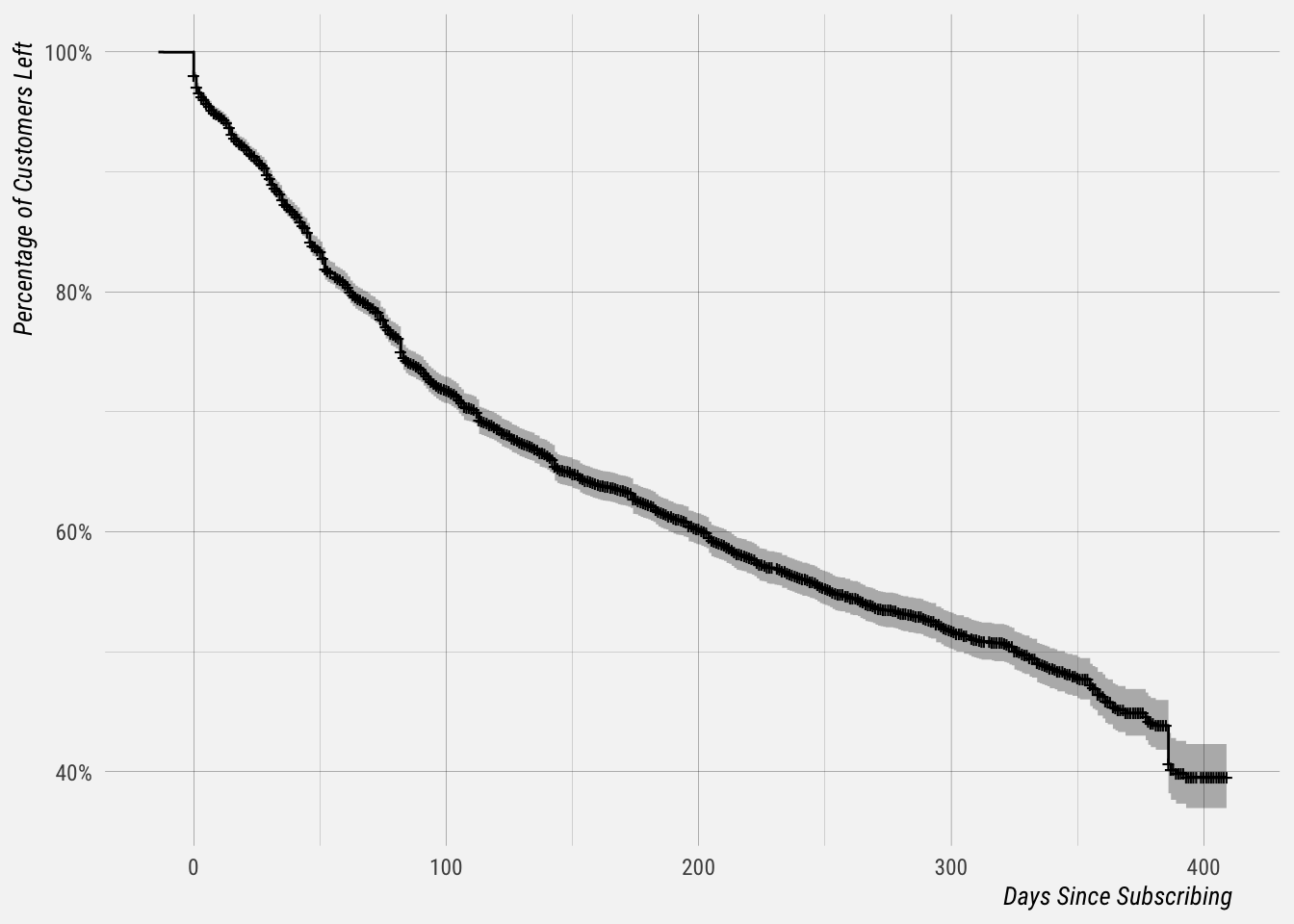
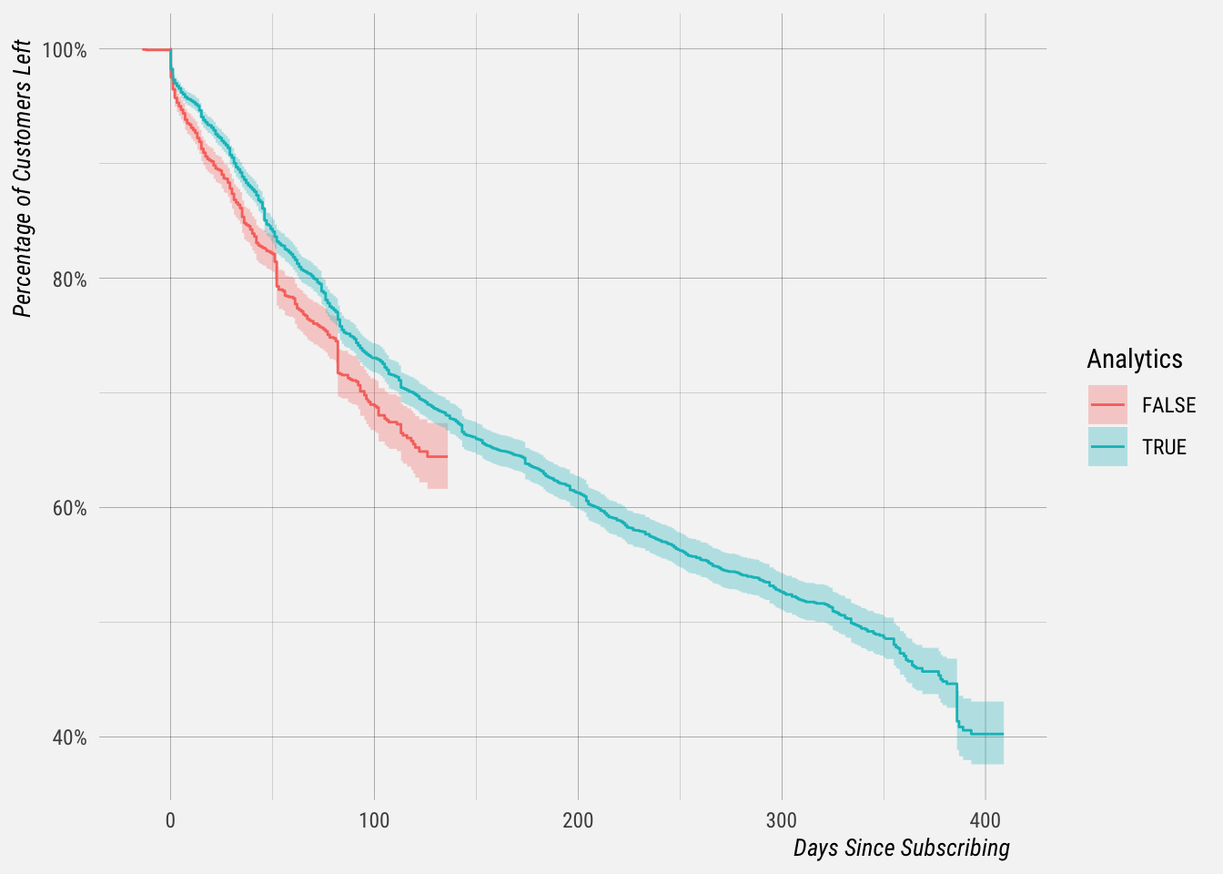
Cool! Now, let’s segment our customers by whether or not they subscribed before we removed Overview analytics from Publish.
# determine whether they had analytics
subs <- subs %>%
  mutate(has_analytics = created_at < "2019-10-01")
Now we can fit survival curves for each segment.
# get survival probabilities
km_fit <- survfit(Surv(days_to_cancel, canceled) ~ has_analytics, data = subs)

# summarise
summary(km_fit, times = c(1, 7, 14, 30, 60, 90, 180))
## Call: survfit(formula = Surv(days_to_cancel, canceled) ~ has_analytics,
## data = subs)
##
## has_analytics=FALSE
## time n.risk n.event survival std.err lower 95% CI upper 95% CI
## 1 2606 94 0.965 0.00356 0.958 0.972
## 7 2420 69 0.938 0.00467 0.929 0.948
## 14 2260 48 0.919 0.00534 0.909 0.930
## 30 1866 103 0.874 0.00670 0.861 0.887
## 60 1275 173 0.783 0.00892 0.765 0.800
## 90 708 94 0.711 0.01078 0.690 0.732
##
## has_analytics=TRUE
## time n.risk n.event survival std.err lower 95% CI upper 95% CI
## 1 4628 126 0.973 0.00235 0.969 0.978
## 7 4524 71 0.958 0.00292 0.952 0.964
## 14 4477 55 0.946 0.00328 0.940 0.953
## 30 4275 194 0.905 0.00427 0.897 0.914
## 60 3867 409 0.818 0.00562 0.808 0.830
## 90 3527 336 0.747 0.00633 0.735 0.760
## 180 2453 517 0.634 0.00708 0.620 0.648It does appear like those customers that had analytics “survived” at higher rates.
Effect of Churn on MRR
# read data from csv
mrr <- read.csv("~/Downloads/biz_mrr.csv", header = T)

# set dates
mrr <- mrr %>%
  mutate(date = as.Date(date, format = "%Y-%m-%d"),
         month = floor_date(date, unit = "months"),
         churn_rate = churn_mrr * -1 / mrr)
Let’s plot the MRR components.
# tidy data
tidy_mrr <- mrr %>%
  mutate(month = floor_date(date, unit = "months"),
         churn_mrr = churn_mrr * -1,
         contraction_mrr = contraction_mrr * -1) %>%
  select(-mrr, -date, -ends_with("customer"), -ends_with("count")) %>%
  gather(type, change, ends_with("mrr")) %>%
  mutate(type = gsub("_mrr", "", type)) %>%
  filter(month != max(month))
Now let’s plot the movements over time.
# plot mrr movements
tidy_mrr %>%
  ggplot(aes(x = month, y = change, color = type)) +
  geom_line() +
  stat_smooth(method = "lm") +
  facet_wrap(~type, scales = "free_y") +
  scale_y_continuous(labels = dollar) +
  theme(legend.position = "none") +
  labs(x = NULL, y = NULL,
       title = "Publish MRR Movements",
       subtitle = "Business Plans Only")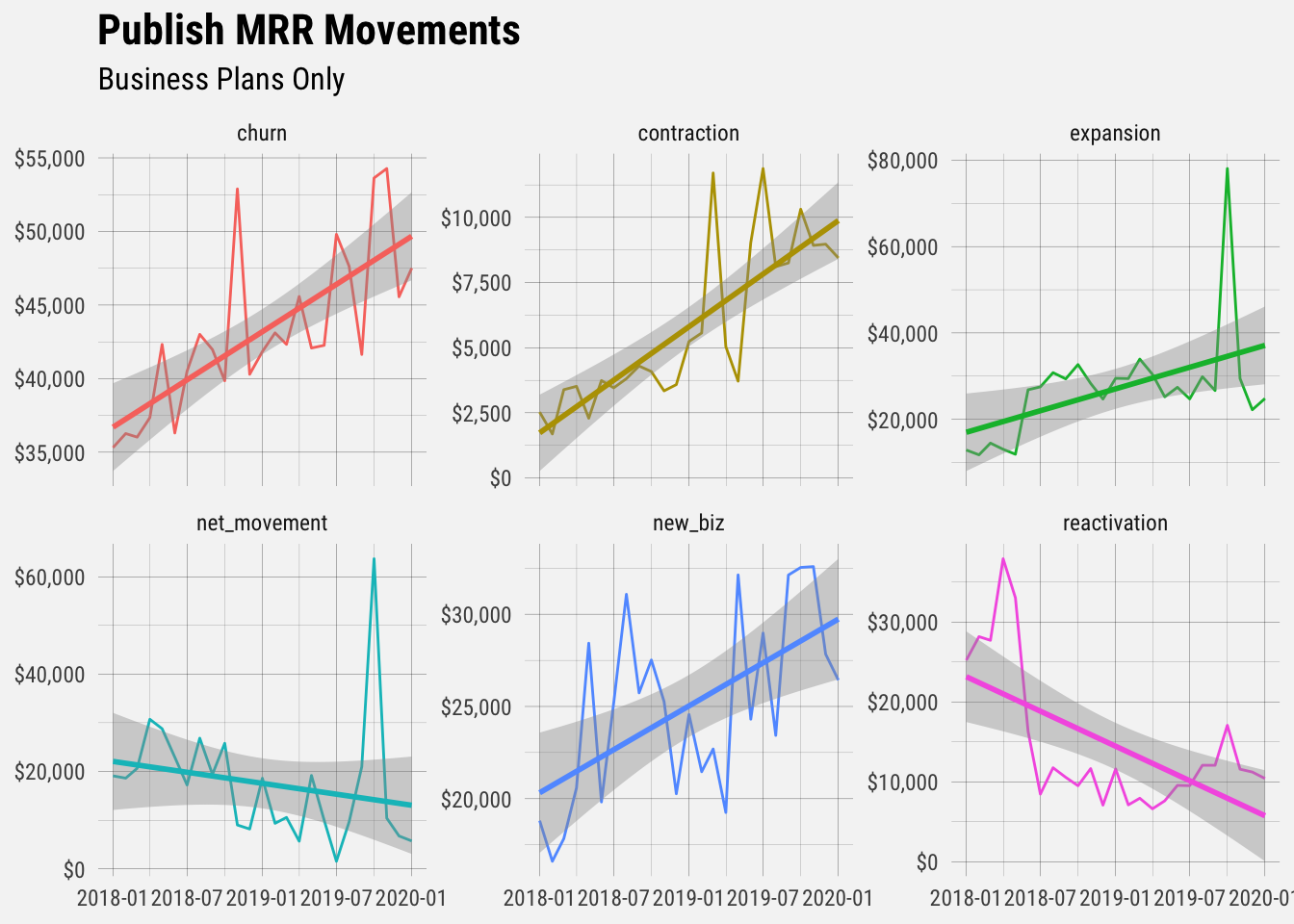
Now let’s get summary stats of the Business churn rate.
# summarise churn rate
mrr %>%
  summarise(avg_churn = mean(churn_rate, na.rm = TRUE),
            sd_churn = sd(churn_rate, na.rm = TRUE),
            first_quartile = quantile(churn_rate, 0.25),
            med_churn = median(churn_rate, na.rm = TRUE),
            third_quartile = quantile(churn_rate, 0.75))
## avg_churn sd_churn first_quartile med_churn third_quartile
## 1 0.04950061 0.005395367 0.047164 0.04889246 0.0521104Let’s plot the churn rate over time. It seems to be relatively stable.
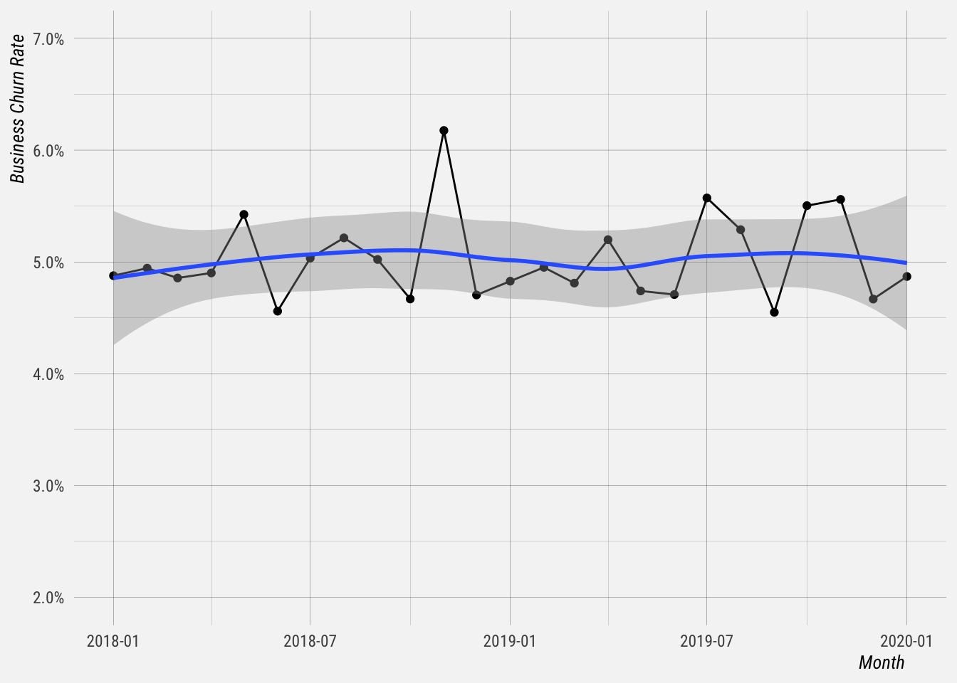
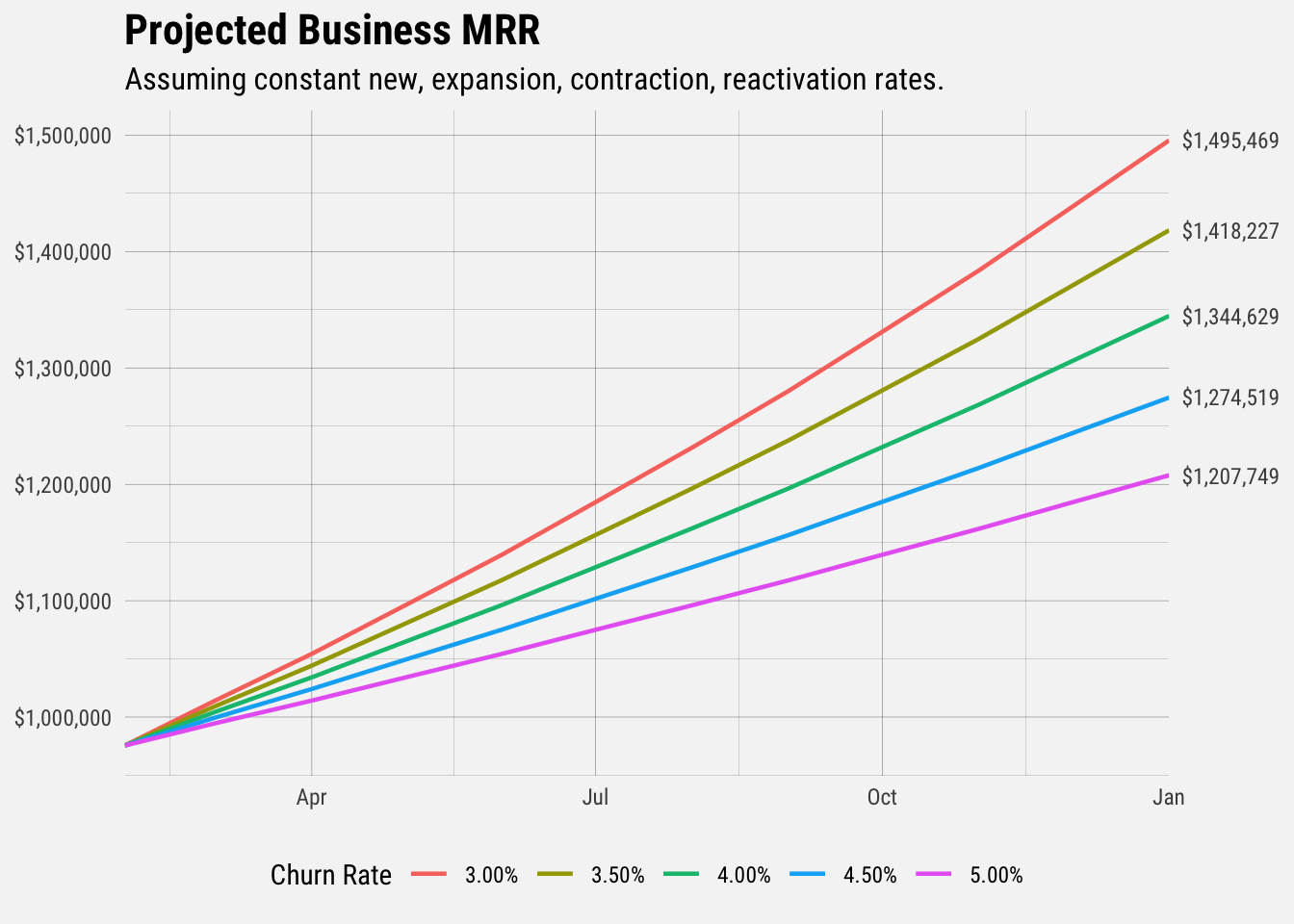
Let’s call the average churn rate 5%. Let’s assume all other rates (new business, contraction, expansion, etc) remain constant.
# get summary stats
mrr_stats <- mrr %>%
  summarise(avg_new = mean(new_biz_mrr / mrr, na.rm = TRUE),
            avg_contraction = mean(contraction_mrr / mrr * -1, na.rm = TRUE),
            avg_expansion = mean(expansion_mrr / mrr, na.rm = TRUE),
            avg_reactivation = mean(reactivation_mrr / mrr, na.rm = TRUE),
            avg_churn = mean(churn_mrr / mrr * -1, na.rm = TRUE))
We’ll use these to project MRR out to the end of 2020.
# get projections for churn rates
get_projections <- function(churn_rate = mrr_stats$avg_churn) {

  # create empty data frame for projections
  projections <- data.frame(month = seq(as.Date("2020-02-01"),
                                        by = "month",
                                        length.out = 24),
                            new = NA,
                            expansion = NA,
                            contraction = NA,
                            reactivation = NA,
                            churn = NA,
                            net = NA,
                            total = 975532.7,
                            churn_rate = NA)
  for (i in 2:24) {

    new <- projections$total[i - 1] * mrr_stats$avg_new
    reactivation <- projections$total[i - 1] * mrr_stats$avg_reactivation
    expansion <- projections$total[i - 1] * mrr_stats$avg_expansion
    contraction <- projections$total[i - 1] * mrr_stats$avg_contraction
    churn <- projections$total[i - 1] * churn_rate
    net <- new + reactivation + expansion - contraction - churn
    total <- projections$total[i - 1] + net

    projections$new[i] <- new
    projections$reactivation[i] <- reactivation
    projections$expansion[i] <- expansion
    projections$contraction[i] <- contraction * -1
    projections$churn[i] <- churn * -1
    projections$net[i] <- net
    projections$total[i] <- total

  }

  projections$churn_rate = as.factor(percent(churn_rate, accuracy = 0.01))

  return(projections)
}

# churn rates to consider
churn_rates <- c(0.03, 0.035, 0.04, 0.045, 0.05)

projections_3 <- get_projections(0.03)
projections_35 <- get_projections(0.035)
projections_4 <- get_projections(0.04)
projections_45 <- get_projections(0.045)
projections_5 <- get_projections(0.05)

forecasts <- rbind(projections_3, projections_35, projections_4, projections_45, projections_5)