Multi-product Homepage Experiment Analysis (EID23)

In this analysis we’ll explore the results from the Multi-Product Homepage Experiment, also known as experimnent EID23. The experiment was run as an A/B test via our A/Bert framework, and split visitors randomly 50/50 between the control and the variation groups.

The experiment hypthosis was:

If we create a new homepage that positions Buffer as a social media platform for DTC brands, and that prominently highlights all three of our products (while keeping the homepage hero CTA pointing to the Publish pricing page), and move the existing homepage to /publish
Then we’ll see an increase in net new MRR
Because new to Buffer users will have a greater awareness of Buffer’s ability to solve many of their social media problems (i.e. analytics and engagement, on top of publishing). They’ll have more context as to what we can do for them, and since Analyze and Reply will be more top of mind, they’ll be more likely to start a trial for more than one product once they start using Buffer.
Please note one small caveat before digging into the results: due to our sunsetting of Reply, and gaps in our instrumentation of Reply, when digging into the per product level this analysis will focus on Publish and Analyze.

TLDR

Visitors to Buffer Accounts Created Ratio: variation is lower, though not statistically significant (barely)
Buffer Accounts to Publish Trials Started Ratio: variation is lower (STAT SIG), but this is a function of fewer signups, as the conversion from signup to trial started had no significant difference
Buffer Accounts to Analyze Trials Started Ratio: variation is higher (STAT SIG)
Publish Trials to Paid Subscription Ratio: variation is higher (not stat sig)
Total Number of Users Converting to a Paid Publish Subscription: variation is higher (not stat sig)
Analyze Trials to Paid Subscription Ratio: variation is higher (not stat sig)
Buffer Account to Multiproduct Paid Subscriptions (Publish & Analyze): variation is higher (STAT SIG), with a total count increase of 17 over the control
Buffer Account to all Paid Subscriptions: variation is higher (not stat sig)
Total MRR generated: variation is higher, with an additional $4274 in MRR, though a sizable chunk of the difference is generated by a small number of users.

The result of the experiment is that there were favorable financial outcomes from the multiproduct homepage. Though we did see a slight drop in Publish signups, which also lead to a slight drop in Publish trials, there was a big increase in Analyze signups and trials started. Though there was a drop in Publish trials started, total users that converted to a Publish paid subscriptions increased slightly, as did the MRR those users generated. Additionally, the number of users that converted to a paid Analyze subscription increased significantly, as did the amount of MRR they generated (though a few users especially so). Total MRR generted by the variant group is impressive, with a 27% increase over the control, but we should proceed with caution in expecting the variant treatment to continue to perform this much better than the control on continued basis given the outsized impact a small number of users had in the variant group.

We recommend enabling the multiproduct homepage for 100% of traffic.

Data Collection

To analyze the results of this experiment, we will use the following query to retrieve data about users enrolled in the experiment.

# connect to bigquery
con <- dbConnect(
  bigrquery::bigquery(),
  project = "buffer-data"
)
# define sql query to get experiment enrolled visitors
sql <- "
  with enrolled_users as (
    select
      anonymous_id
      , experiment_group
      , first_value(timestamp) over (
      partition by anonymous_id order by timestamp asc
      rows between unbounded preceding and unbounded following) as enrolled_at
    from segment_marketing.experiment_viewed
    where 
      first_viewed 
      and experiment_id = 'eid23_multi_product_homepage'
      and timestamp >= '2020-02-14'
      and timestamp < '2020-02-28'
  )
  select
    e.anonymous_id
    , e.experiment_group
    , e.enrolled_at
    , i.user_id as account_id
    , c.email
    , c.publish_user_id
    , c.analyze_user_id
    , a.timestamp as account_created_at
    , t.product as trial_product
    , t.timestamp as trial_started_at
    , t.subscription_id as trial_subscription_id
    , t.stripe_event_id as stripe_trial_event_id
    , t.plan_id as trial_plan_id
    , t.cycle as trial_billing_cycle
    , t.cta as trial_started_cta
    , s.product as subscription_product
    , s.timestamp as subscription_started_at
    , s.subscription_id as subscription_id
    , s.stripe_event_id as stripe_subscription_event_id
    , s.plan_id as subscription_plan_id
    , s.cycle as subscritpion_billing_cycle
    , s.revenue as subscription_revenue
    , s.amount as subscritpion_amount
    , s.cta as subscription_started_cta
  from enrolled_users e
    left join segment_login_server.identifies i
      on e.anonymous_id = i.anonymous_id
    left join dbt_buffer.core_accounts c
      on i.user_id = c.id
    left join segment_login_server.account_created a
      on i.user_id = a.user_id
    left join segment_publish_server.trial_started t
      on i.user_id = t.user_id
      and t.timestamp > e.enrolled_at
    left join segment_publish_server.subscription_started s
      on i.user_id = s.user_id
      and s.timestamp > e.enrolled_at
  group by 1,2,3,4,5,6,7,8,9,10,11,12,13,14,15,16,17,18,19,20,21,22,23,24
"
  
# query BQ
# users <- dbGetQuery(con, sql)

Analysis

Let’s start the analysis by reviewing a few of the summary statistics from our data.

skim(users)

## Skim summary statistics
##  n obs: 211073 
##  n variables: 24 
## 
## ── Variable type:character ───────────────────────────────
##                      variable missing complete      n min max empty
##                    account_id  192989    18084 211073  24  24     0
##               analyze_user_id  208909     2164 211073  24  24     0
##                  anonymous_id       0   211073 211073  36  36     0
##                         email  193713    17360 211073   8  48     0
##              experiment_group       0   211073 211073   7   9     0
##               publish_user_id  193860    17213 211073  24  24     0
##  stripe_subscription_event_id  209950     1123 211073  18  28     0
##         stripe_trial_event_id  200736    10337 211073  18  28     0
##               subscription_id  209950     1123 211073  18  18     0
##          subscription_plan_id  209950     1123 211073  13  44     0
##          subscription_product  209950     1123 211073   7   7     0
##      subscription_started_cta  210031     1042 211073  30  75     0
##    subscritpion_billing_cycle  209950     1123 211073   4   5     0
##           trial_billing_cycle  200736    10337 211073   4   5     0
##                 trial_plan_id  200736    10337 211073  13  44     0
##                 trial_product  200736    10337 211073   7   7     0
##             trial_started_cta  200790    10283 211073  30  75     0
##         trial_subscription_id  200736    10337 211073  18  18     0
##  n_unique
##     16994
##      1333
##    209617
##     16325
##         2
##     16178
##       931
##     10214
##       930
##        15
##         2
##        44
##         2
##         2
##        14
##         2
##        46
##     10019
## 
## ── Variable type:integer ─────────────────────────────────
##              variable missing complete      n  mean     sd p0 p25 p50 p75
##  subscription_revenue  209950     1123 211073 31.82  32.22 12  15  15  50
##   subscritpion_amount  209950     1123 211073 90.02 172    15  15  35  99
##  p100     hist
##   399 ▇▁▁▁▁▁▁▁
##  2030 ▇▁▁▁▁▁▁▁
## 
## ── Variable type:POSIXct ─────────────────────────────────
##                 variable missing complete      n        min        max
##       account_created_at  192990    18083 211073 2019-04-23 2020-03-23
##              enrolled_at       0   211073 211073 2020-02-14 2020-02-27
##  subscription_started_at  209950     1123 211073 2020-02-14 2020-03-23
##         trial_started_at  200736    10337 211073 2020-02-14 2020-03-23
##      median n_unique
##  2020-02-17    16993
##  2020-02-19   209592
##  2020-03-03      931
##  2020-02-21    10216

We can now do a quick validation of the visitor count split between the two experiment groups.

users %>% 
  group_by(experiment_group) %>% 
  summarise(visitors = n_distinct(anonymous_id)) %>% 
  mutate(visitor_split_perct = visitors / sum(visitors)) %>%
  kable() %>% 
  kable_styling()

experiment_group	visitors	visitor_split_perct
control	104611	0.4990578
variant_1	105006	0.5009422

Great, there is a total of 209,617 unique visitors enrolled in the experiment, and the percentage split between the two experiment groups is within a few hundred visitors of exactly 50/50. This confirms that our experiment framework correctly split enrollments for the experiment. Next, we will run a proportion test to see if there was a satistical signicant difference is the visitor to signup ratio between the two groups.

users %>% 
  group_by(experiment_group) %>% 
  summarise(accouts = n_distinct(account_id)) %>% 
  kable() %>% 
  kable_styling()

experiment_group	accouts
control	8602
variant_1	8394

res <- prop.test(x = c(8602, 8394), n = c(104611, 105006), alternative = "two.sided")
res

## 
##  2-sample test for equality of proportions with continuity
##  correction
## 
## data:  c(8602, 8394) out of c(104611, 105006)
## X-squared = 3.6582, df = 1, p-value = 0.05579
## alternative hypothesis: two.sided
## 95 percent confidence interval:
##  -5.645027e-05  4.636764e-03
## sample estimates:
##     prop 1     prop 2 
## 0.08222845 0.07993829

We can see that the number of visitors that ended up creating a Buffer account (ie, signed up for their first Buffer product), was a few hundred higher in the control group. Using a quick proportion test we can see that this difference in proportion of enrolled visitors that created a Buffer account is NOT statistically significant, with a p-value of 0.056 (which is just barely over the generally accepted 0.05 threshold).

Next, we will calculate how many users from each experiment group started a trial for each product.

users %>% 
  mutate(has_publish_trial = trial_product == "publish") %>% 
  group_by(experiment_group, has_publish_trial) %>% 
  summarise(users = n_distinct(account_id)) %>% 
  ungroup() %>% 
  filter(has_publish_trial) %>% 
  group_by(experiment_group) %>% 
  summarise(users_with_publish_trials = users) %>%
  kable() %>% 
  kable_styling()

experiment_group	users_with_publish_trials
control	4620
variant_1	4432

There were 4620 users in the control group that started a Publish trial, and 4432 in the variation group. Just like above, we should also run a proportion test here.

res <- prop.test(x = c(4620, 4432), n = c(8602, 8394), alternative = "two.sided")
res

## 
##  2-sample test for equality of proportions with continuity
##  correction
## 
## data:  c(4620, 4432) out of c(8602, 8394)
## X-squared = 1.3733, df = 1, p-value = 0.2412
## alternative hypothesis: two.sided
## 95 percent confidence interval:
##  -0.006032226  0.024208648
## sample estimates:
##    prop 1    prop 2 
## 0.5370844 0.5279962

We can see that the difference in proportion of accounts that started a Publish trial is also NOT statistically significant, with a p-value of 0.241. This is to be expected though, given the vast majority of Publish signups via web are through workflows that start trials.

Now let’s look at Analyze trial starts per group.

users %>% 
  mutate(has_analyze_trial = (trial_product == "analyze")) %>% 
  group_by(experiment_group, has_analyze_trial) %>% 
  summarise(users = n_distinct(account_id)) %>% 
  ungroup() %>% 
  filter(has_analyze_trial) %>% 
  group_by(experiment_group) %>% 
  summarise(users_with_analyze_trials = users) %>%
  kable() %>% 
  kable_styling()

experiment_group	users_with_analyze_trials
control	382
variant_1	476

There were 382 users in the control group that started an Analyze trial, and 476 in the variation group. Just like above, we should also run a proportion test here.

res <- prop.test(x = c(382, 476), n = c(8602, 8394), alternative = "two.sided")
res

## 
##  2-sample test for equality of proportions with continuity
##  correction
## 
## data:  c(382, 476) out of c(8602, 8394)
## X-squared = 13.151, df = 1, p-value = 0.0002874
## alternative hypothesis: two.sided
## 95 percent confidence interval:
##  -0.019006811 -0.005590978
## sample estimates:
##     prop 1     prop 2 
## 0.04440828 0.05670717

We can see that the difference in proportion of accounts that started an Analyze trial IS statistically significant, with a p-value of 0.0003 (which is much less than the generally accepted 0.05 threshold). This means we can say with confidence that the observed difference in the number of Analyze trials started between the two experiment groups was not the result of random variance.

Next, we will calculate how many users from each experiment group started a paid subscription from each product.

users %>% 
  mutate(has_publish_sub = (subscription_product == "publish")) %>% 
  group_by(experiment_group, has_publish_sub) %>% 
  summarise(users = n_distinct(account_id)) %>% 
  ungroup() %>% 
  filter(has_publish_sub) %>% 
  group_by(experiment_group) %>% 
  summarise(paying_publish_users = users) %>%
  kable() %>% 
  kable_styling()

experiment_group	paying_publish_users
control	391
variant_1	408

There were 391 users in the control group that started a paid Publish subscription, and 408 in the variation group. Just like above, we should also run a proportion test here, for both the account to paid subscription proportion, and also the trial to paid subscription proportion.

res <- prop.test(x = c(391, 408), n = c(8602, 8394), alternative = "two.sided")
res

## 
##  2-sample test for equality of proportions with continuity
##  correction
## 
## data:  c(391, 408) out of c(8602, 8394)
## X-squared = 0.87285, df = 1, p-value = 0.3502
## alternative hypothesis: two.sided
## 95 percent confidence interval:
##  -0.009636347  0.003333144
## sample estimates:
##     prop 1     prop 2 
## 0.04545455 0.04860615

There is no statistical difference between the two proportions of accounts that started a paid Publish subscription, as the p-value is 0.350.

res <- prop.test(x = c(391, 408), n = c(4620, 4432), alternative = "two.sided")
res

## 
##  2-sample test for equality of proportions with continuity
##  correction
## 
## data:  c(391, 408) out of c(4620, 4432)
## X-squared = 1.459, df = 1, p-value = 0.2271
## alternative hypothesis: two.sided
## 95 percent confidence interval:
##  -0.019345519  0.004494064
## sample estimates:
##     prop 1     prop 2 
## 0.08463203 0.09205776

There is no statistical difference between the two proportions of Publish trialists that started a paid Publish subscription, as the p-value is 0.227.

Next, let’s look into the number of Analyze paid subscriptions between the two experiment groups.

users %>% 
  mutate(has_analyze_sub = (subscription_product == "analyze")) %>% 
  group_by(experiment_group, has_analyze_sub) %>% 
  summarise(users = n_distinct(account_id)) %>% 
  ungroup() %>% 
  filter(has_analyze_sub) %>% 
  group_by(experiment_group) %>% 
  summarise(paying_publish_users = users) %>%
  kable() %>% 
  kable_styling()

experiment_group	paying_publish_users
control	50
variant_1	76

The number of paying users for Analyze was 50 in the control and 76 in the variation. Just like above, we should also run a couple of proportion tests here too.

res <- prop.test(x = c(50, 76), n = c(8602, 8394), alternative = "two.sided")
res

## 
##  2-sample test for equality of proportions with continuity
##  correction
## 
## data:  c(50, 76) out of c(8602, 8394)
## X-squared = 5.6337, df = 1, p-value = 0.01762
## alternative hypothesis: two.sided
## 95 percent confidence interval:
##  -0.0059450453 -0.0005379238
## sample estimates:
##      prop 1      prop 2 
## 0.005812602 0.009054086

The variation group DID have a statisticaly significant increase in proportion of Analyze Paid Subscriptions, with a p-value of 0.018.

res <- prop.test(x = c(50, 76), n = c(382, 476), alternative = "two.sided")
res

## 
##  2-sample test for equality of proportions with continuity
##  correction
## 
## data:  c(50, 76) out of c(382, 476)
## X-squared = 1.1802, df = 1, p-value = 0.2773
## alternative hypothesis: two.sided
## 95 percent confidence interval:
##  -0.07832180  0.02077418
## sample estimates:
##    prop 1    prop 2 
## 0.1308901 0.1596639

There is no statistical difference between the two proportions of Analyze trials that started a paid Analyze subscription, as the p-value is 0.277. This means that the difference in paid Analyze subscriptions is more the result of an increase in Analyze trials started in the variation group, not a statistically significant increase in the conversion rate to paid between the two groups.

Next, we will look at the number of accounts that started paid subscriptions for both Publish and Analyze in both experiment groups.

users %>% 
  filter(!is.na(subscription_product)) %>% 
  group_by(account_id, experiment_group) %>% 
  summarise(products = n_distinct(subscription_product)) %>% 
  ungroup() %>% 
  filter(products > 1) %>% 
  group_by(experiment_group, products) %>% 
  summarise(users = n_distinct(account_id)) %>%
  kable() %>% 
  kable_styling()

experiment_group	products	users
control	2	29
variant_1	2	46

res <- prop.test(x = c(29, 46), n = c(8602, 8394), alternative = "two.sided")
res

## 
##  2-sample test for equality of proportions with continuity
##  correction
## 
## data:  c(29, 46) out of c(8602, 8394)
## X-squared = 3.8337, df = 1, p-value = 0.05023
## alternative hypothesis: two.sided
## 95 percent confidence interval:
##  -4.225154e-03  7.562313e-06
## sample estimates:
##      prop 1      prop 2 
## 0.003371309 0.005480105

There IS a statistical difference between the two proportions of accounts started in each experiment group that ended up starting both a paid Analyze subscription and a paid Publish subscription, with a p-value of 0.050 (just squeaking inside the the generally accepted .05 threshold of significance when rounded). It does appear that the variation lead to more users on paid subscriptions for both Publish and Analyze.

Finally, let’s also look at the MRR value of all converted trials per experiment group, to see if there was any overall difference in value between the two groups.

MRR Per Experiment Group

To start the comparison in MRR generated by each of the two experiment groups, let’s look at some summary statistics.

mrr <- users %>% 
  mutate(mrr_value = subscription_revenue) %>% 
  select(account_id, experiment_group, mrr_value) %>% 
  group_by(account_id, experiment_group) %>% 
  summarise(mrr_value = sum(mrr_value))

summary_by_group <- mrr %>% 
  group_by(experiment_group) %>%
  summarise(
    unique_users = n_distinct(account_id),
    paid_users = sum(if_else(mrr_value > 0, 1, 0), na.rm = TRUE),
    conv_rate = (sum(if_else(mrr_value > 0, 1, 0), na.rm = TRUE) / n_distinct(account_id)),
    min_mrr = min(mrr_value, na.rm = TRUE),
    max_mrr = max(mrr_value, na.rm = TRUE),
    median_mrr = median(mrr_value, na.rm = TRUE),
    mean_mrr = mean(mrr_value, na.rm = TRUE),
    sum_mrr = sum(mrr_value, na.rm = TRUE),
    std_dev_mrr = sd(mrr_value, na.rm = TRUE),
    ) %>% 
  mutate(pct_change_mrr = ((sum_mrr - lag(sum_mrr)) / lag(sum_mrr)) * 100) %>% 
  gather(key = "key", value = "value", 2:11) %>% 
  spread(key = "experiment_group", value = "value") %>% 
  arrange(desc(key)) %>% 
  rename(metric = key) %>% 
  kable(digits = 2) %>%
  kable_styling(bootstrap_options = c("striped", "hover", "condensed"))
summary_by_group

metric	control	variant_1
unique_users	8602.00	8394.00
sum_mrr	15731.00	20005.00
std_dev_mrr	53.97	75.34
pct_change_mrr	NA	27.17
paid_users	412.00	438.00
min_mrr	12.00	12.00
median_mrr	15.00	15.00
mean_mrr	38.18	45.67
max_mrr	447.00	897.00
conv_rate	0.05	0.05

Right off the top, we can see that the variation group generated $4,274 more in MRR than the control, which was a 27% improvement. The variation group also had an increase in the number of paid users, with an additional 26. Given this, we should next examine if there is a statistical difference between the number of Buffer signups that converted to a paid subscription.

res <- prop.test(x = c(412, 438), n = c(8602, 8394), alternative = "two.sided")
res

## 
##  2-sample test for equality of proportions with continuity
##  correction
## 
## data:  c(412, 438) out of c(8602, 8394)
## X-squared = 1.5524, df = 1, p-value = 0.2128
## alternative hypothesis: two.sided
## 95 percent confidence interval:
##  -0.010959313  0.002390732
## sample estimates:
##     prop 1     prop 2 
## 0.04789584 0.05218013

With a p-value of 0.213 the observed difference with paid users is not statistically significant. This indicates that though the Buffer signup to paid conversion rate increased, as did the difference in observed MRR generated by the variation group, this might be attributed to a small number of users and natural variance can not be ruled out. This is additionally supported by the higher standard deviation of MRR in the variation group.

Let’s take a quick look at a box plot to see the distribution of MRR amounts within each experiment group. The box plot will give us a quick over view of the each experiment groups central tendency and spread.

ggboxplot(mrr, x = "experiment_group", y = "mrr_value", 
          color = "experiment_group", palette = c("#00AFBB", "#E7B800"),
          ylab = "mrr_value", xlab = "experiment_group")

## Warning: Removed 16146 rows containing non-finite values (stat_boxplot).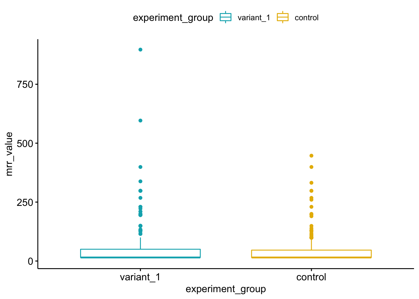

We can see in the above blox plot graph that the variation group has a few larger max values, which will impact the the MRR mean, but also what looks like perhaps more clustering higher above the 75 percentile. This indicates that the difference in paid subscription behavior between the two groups is very similar, and that the observed differences are likely attributed to a smaller group in the variation group (perhaps the additional 17 users on paid subscriptions for both products). We can dig into this just a little bit more by looking at the MRR amount by experiment group, visualized by density.

ggdensity(mrr, x = "mrr_value", add = "mean", rug = TRUE,
          color = "experiment_group", fill = "experiment_group", facet.by = "experiment_group", palette = c("#E7B800", "#00AFBB"),
          ylab = "Density", xlab = "MRR Amount")

## Warning: Removed 16146 rows containing non-finite values (stat_density).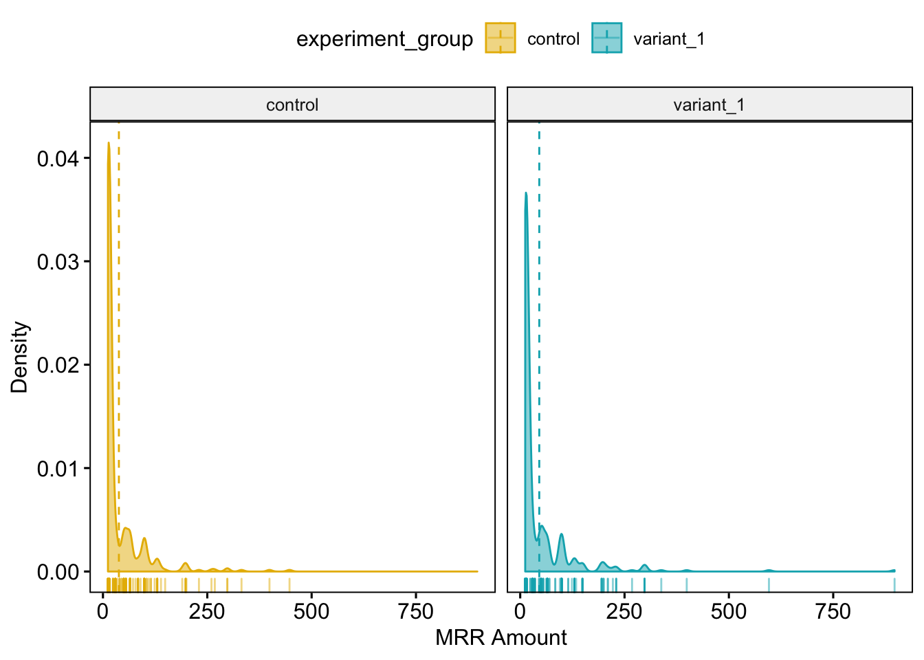

We can see that the two groups have some similarities in general shape, but with densities shifted more to the right in the variation group. This can especially be seen in the tick marks along the X axis. This makes sense given the additional 17 users on both Publish and Analyze paid subscriptions in the Variation group.

In order to test this change in density for statistical significance, we will look at the MRR per signup, which will account for differences in MRR where either more users purchased a lower price plan or fewer purchased at a higher priced plan. In order to do this, we will run a Mann Whitney Wilcoxon Test, which is a statistical hypothesis test that is the non-parametric equivalent to the t-test, and DOES NOT require data to be normally distributed.

The Null Hypothesis is that the difference between the two populations is zero (i.e. there is no difference.) The Alternative Hypothesis is that the difference between the two populations is not zero (i.e. there is a difference.)

result <- wilcox.test(mrr_value ~ experiment_group, data = mrr,
            conf.int = TRUE, conf.level = 0.95)
result

## 
##  Wilcoxon rank sum test with continuity correction
## 
## data:  mrr_value by experiment_group
## W = 86370, p-value = 0.2531
## alternative hypothesis: true location shift is not equal to 0
## 95 percent confidence interval:
##  -2.901880e-05  2.166157e-05
## sample estimates:
## difference in location 
##           -4.68477e-05

With a p-value of 0.253, the difference between the two experiment groups is NOT statistically significant, which indicates that the $7.49 greater MRR per paid user observed in the variant group has a 1 out of 4 chance of occurring from natural variance. This is likely a result of a small number of users generating a disproporiate amount of the variantion group’s MRR.

Bottom line, there is an observed 27% increase in MRR generated by the variation group, but that increase in MRR is not driven by enough users to entirely rule out natural variance as the cause.

Let’s also take a per product view of MRR, to see if we can get a more complete picture of this impact a few higher value customers might be having on the comnparison of MRR between the two groups.

mrr_by_product <- users %>% 
  mutate(mrr_value = subscription_revenue) %>% 
  unite(group_and_product, c("experiment_group", "subscription_product")) %>% 
  group_by(account_id, group_and_product) %>% 
  summarise(mrr_value = sum(mrr_value))

summary_by_group <- mrr_by_product %>% 
  filter(!is.na(mrr_value)) %>% 
  group_by(group_and_product) %>%
  summarise(
    paid_users = sum(if_else(mrr_value > 0, 1, 0), na.rm = TRUE),
    min_mrr = min(mrr_value, na.rm = TRUE),
    max_mrr = max(mrr_value, na.rm = TRUE),
    median_mrr = median(mrr_value, na.rm = TRUE),
    mean_mrr = mean(mrr_value, na.rm = TRUE),
    sum_mrr = sum(mrr_value, na.rm = TRUE),
    std_dev_mrr = sd(mrr_value, na.rm = TRUE),
    ) %>% 
  gather(key = "key", value = "value", 2:8) %>% 
  spread(key = "group_and_product", value = "value") %>% 
  arrange(desc(key)) %>% 
  rename(metric = key) %>% 
  kable(digits = 2) %>%
  kable_styling(bootstrap_options = c("striped", "hover", "condensed"))
summary_by_group

metric	control_analyze	control_publish	variant_1_analyze	variant_1_publish
sum_mrr	3305.00	12426.00	6126.00	13879.00
std_dev_mrr	28.14	43.62	71.38	48.42
paid_users	50.00	391.00	76.00	408.00
min_mrr	35.00	12.00	28.00	12.00
median_mrr	50.00	15.00	50.00	15.00
mean_mrr	66.10	31.78	80.61	34.02
max_mrr	150.00	399.00	600.00	399.00

We can see that the variant group generated more MRR and had more paying customers (as stated previously in this analysis) for each product, compared to the control group.

Let’s now look at a box plot for this per product MRR dataframe.

mrr_by_product_1 <- mrr_by_product %>% 
  filter(!is.na(mrr_value))

ggboxplot(mrr_by_product_1, x = "group_and_product", y = "mrr_value", 
          color = "group_and_product",
          ylab = "mrr_value", xlab = "group_and_product")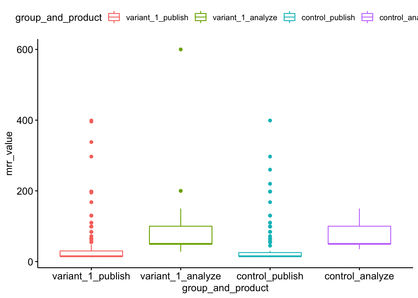

With this box plot, we can see the three outliers for Analyze subscriptions in the variant group that are providing an oversized contribution to the mean (there are two subscriptions at the $200 MRR mark, though only one dot plotted). These 3 Analyze subscriptions in the variant group comprise 25% of the additional MRR generated by the variant group over the control group. This indicates that we should proceed with caution in expecting the treatment to generate this much additional MRR on a continued basis, as a sizable portion is depended on only a few subscriptions.

Final Thoughts

Given the above observations, the result of the experiment is that there were favorable financial outcomes from the multiproduct homepage. Though we did see a drop in Publish signups, which also lead to a drop in Publish trials, there was a big increase in Analyze signups and trials started. Though there was a drop in Publish trials started, total users that converted to a Publish paid subscriptions increased slightly, as did the MRR those users generated. Additionally, the number of users that converted to a paid Analyze subscription increased significantly, as did the amount of MRR they generated (though a few users especially so). Total MRR generted by the variant group is impressive, with a 27% increase over the control, but we should proceed with caution in expecting the variant treatment to continue to perform this much better than the control on an on going basis given the outsized impact a few users had in the variant group.

We recommend enabling the multiproduct homepage for 100% of traffic.