In this analysis we’ll explore the results from the Product Solutions V2 Experiment, also known as experiment EID22. The experiment was run as an A/B test via our A/Bert framework, and split visitors randomly 50/50 between the control and the variation groups.
The experiment hypothesis was:
If we replace the content on /business with content promoting the solution of Publish and Analyze bundled together, starting trials for both products as the same time via one workflow (with the focus on $85/mo Premium product solution through all the CTA buttons and less explicitly the $50/mo Pro product solution in the FAQ)*
Then we will see an increase in net new MRR from new-to-Buffer users
Because we believe the product solutions are more valuable and suitable for more prospects than the Publish Small Business plan, the product solutions are inline with our multi-product strategy, and the Publish Small Business plan will be folded into the Publish Premium plan eventually.
Please note that visitors were enrolled in the experiment upon landing on
/business, but they could have ended up signing up from another page (IE, they did not have to signup for a bundle solution to be included in the experiment results)
TLDR
Of users/visitors enrolled in the experiment (IE, visited /business at least once prior to account creation and during the experiment), we observed the following differences between the two groups:
- Visitors to Buffer Accounts Created Ratio: not statistically significant (not stat sig), variation is slightly lower
- Visitors to Publish Trials Started Ratio: not stat sig, variation is slightly lower
- Visitors to Analyze Trials Started Ratio: variation is higher (STAT SIG), increasing from 3% to 21%
- Publish Trials to Paid Subscription Ratio: not stat sig, no difference
- Total Number of Users Converting to a Paid Publish Subscription: not stat sig, no difference
- Analyze Trials to Paid Subscription Ratio: variation is lower (STAT SIG), conversion rate dropped from 9% to 3%, though the total number of paid Analyze Subscriptions was stat sig higher in the variation group
- Total Number of Users Converting to a Paid Analyze Subscription: variation is higher (STAT SIG), increasing from 15 users to 35 users
- Buffer Account to Multiple Product Paid Subscriptions (Publish & Analyze): variation is higher (STAT SIG), with a total count increase of 22 users over the control
- Buffer Account to all Paid Subscriptions Rate: not stat sig, no difference
- Total MRR Generated: variation is higher, with an additional $1486 in MRR (a 49% increase).
The result of the experiment is that there were favorable financial outcomes from the variation treatment changes made to the /business page. Though we did see a small drop in Publish trials started, there was a big increase in Analyze trials started. Even with this slight drop in Publish trials started, total number of users that converted to a Publish paid subscriptions increased slightly, as did the MRR those users generated. Additionally, the number of users that converted to a paid Analyze subscription increased significantly, as did the amount of MRR they generated. Total MRR generated by the variant group was $1486 more than the control group, which was a 49% increase.
We recommend enabling the Solutions V2 treatment changes for 100% of traffic.
Data Collection
To analyze the results of this experiment, we will use the following query to retrieve data about users enrolled in the experiment.
# connect to bigquery
con <- dbConnect(
  bigrquery::bigquery(),
  project = "buffer-data"
)
# define sql query to get experiment enrolled visitors
sql <- "
  with enrolled_users as (
    select
      anonymous_id
      , experiment_group
      , first_value(timestamp) over (
      partition by anonymous_id order by timestamp asc
      rows between unbounded preceding and unbounded following) as enrolled_at
    from segment_marketing.experiment_viewed
    where
      first_viewed
      and experiment_id = 'eid22_analyze_publish_product_solution_v2'
      and timestamp >= '2020-03-02'
      and timestamp <= '2020-03-16'
  )
  select
    e.anonymous_id
    , e.experiment_group
    , e.enrolled_at
    , i.user_id as account_id
    , c.email
    , c.publish_user_id
    , c.analyze_user_id
    , a.timestamp as account_created_at
    , t.product as trial_product
    , t.timestamp as trial_started_at
    , t.subscription_id as trial_subscription_id
    , t.stripe_event_id as stripe_trial_event_id
    , t.plan_id as trial_plan_id
    , t.cycle as trial_billing_cycle
    , t.cta as trial_started_cta
    , s.product as subscription_product
    , s.timestamp as subscription_started_at
    , s.subscription_id as subscription_id
    , s.stripe_event_id as stripe_subscription_event_id
    , s.plan_id as subscription_plan_id
    , s.cycle as subscritpion_billing_cycle
    , s.revenue as subscription_revenue
    , s.amount as subscritpion_amount
    , s.cta as subscription_started_cta
  from enrolled_users e
    left join segment_login_server.identifies i
      on e.anonymous_id = i.anonymous_id
    left join dbt_buffer.core_accounts c
      on i.user_id = c.id
    left join segment_login_server.account_created a
      on i.user_id = a.user_id
    left join segment_publish_server.trial_started t
      on i.user_id = t.user_id
      and t.timestamp > e.enrolled_at
    left join segment_publish_server.subscription_started s
      on i.user_id = s.user_id
      and s.timestamp > e.enrolled_at
  group by 1,2,3,4,5,6,7,8,9,10,11,12,13,14,15,16,17,18,19,20,21,22,23,24
"

# query BQ
# users <- dbGetQuery(con, sql)
Analysis
Let’s start the analysis by reviewing a few of the summary statistics from our data.
skim(users)## Skim summary statistics
## n obs: 11748
## n variables: 24
##
## ── Variable type:character ───────────────────────────────
## variable missing complete n min max empty
## account_id 6805 4943 11748 24 24 0
## analyze_user_id 9248 2500 11748 24 24 0
## anonymous_id 0 11748 11748 36 36 0
## email 7081 4667 11748 10 48 0
## experiment_group 0 11748 11748 7 9 0
## publish_user_id 7103 4645 11748 24 24 0
## stripe_subscription_event_id 11408 340 11748 18 28 0
## stripe_trial_event_id 7184 4564 11748 18 28 0
## subscription_id 11408 340 11748 18 18 0
## subscription_plan_id 11408 340 11748 13 44 0
## subscription_product 11408 340 11748 7 7 0
## subscription_started_cta 11424 324 11748 30 75 0
## subscritpion_billing_cycle 11408 340 11748 4 5 0
## trial_billing_cycle 7184 4564 11748 4 5 0
## trial_plan_id 7184 4564 11748 13 44 0
## trial_product 7184 4564 11748 7 7 0
## trial_started_cta 7201 4547 11748 30 75 0
## trial_subscription_id 7184 4564 11748 18 18 0
## n_unique
## 3575
## 1246
## 10271
## 3361
## 2
## 3339
## 228
## 4481
## 228
## 10
## 2
## 26
## 2
## 2
## 11
## 2
## 38
## 4433
##
## ── Variable type:integer ─────────────────────────────────
## variable missing complete n mean sd p0 p25 p50 p75
## subscription_revenue 11408 340 11748 36.21 26.5 12 15 28 50
## subscritpion_amount 11408 340 11748 69.93 107.64 15 15 50 65
## p100 hist
## 99 ▇▁▂▅▁▁▁▂
## 663 ▇▂▁▁▁▁▁▁
##
## ── Variable type:POSIXct ─────────────────────────────────
## variable missing complete n min max
## account_created_at 6805 4943 11748 2019-04-26 2020-04-10
## enrolled_at 0 11748 11748 2020-03-02 2020-03-15
## subscription_started_at 11408 340 11748 2020-03-02 2020-04-10
## trial_started_at 7184 4564 11748 2020-03-02 2020-04-10
## median n_unique
## 2020-03-08 3575
## 2020-03-09 10271
## 2020-03-23 228
## 2020-03-09 4481We can now do a quick validation of the visitor count split between the two experiment groups.
users %>%
  group_by(experiment_group) %>%
  summarise(visitors = n_distinct(anonymous_id)) %>%
  mutate(visitor_split_perct = visitors / sum(visitors)) %>%
  kable() %>%
kable_styling()| experiment_group | visitors | visitor_split_perct |
|---|---|---|
| control | 5107 | 0.4972252 |
| variant_1 | 5164 | 0.5027748 |
Great, there is a total of 10271 unique visitors enrolled in the experiment, and the percentage split between the two experiment groups is about a quarter of a percentage point of exactly 50/50 (a little deviance from 50/50 split is expected from the randomization). This confirms that our experiment framework correctly split enrollments for the experiment. Next, we will run a proportion test to see if there was a statistical significant difference is the visitor to signup ratio between the two groups.
users %>%
  group_by(experiment_group) %>%
  summarise(accouts = n_distinct(account_id)) %>%
  kable() %>%
kable_styling()| experiment_group | accouts |
|---|---|
| control | 1797 |
| variant_1 | 1780 |
res <- prop.test(x = c(1797, 1780), n = c(5107, 5164), alternative = "two.sided")
res
##
## 2-sample test for equality of proportions with continuity
## correction
##
## data: c(1797, 1780) out of c(5107, 5164)
## X-squared = 0.55134, df = 1, p-value = 0.4578
## alternative hypothesis: two.sided
## 95 percent confidence interval:
## -0.01144632 0.02579821
## sample estimates:
## prop 1 prop 2
## 0.351870 0.344694We can see that the number of visitors that ended up creating a Buffer account (IE, signed up for their first Buffer product), was a little higher in the control group. Using a quick proportion test we can see that this difference in proportion of enrolled visitors that created a Buffer account is NOT statistically significant, with a p-value of 0.4578. Thus, the observed difference in signups is likely due to natural variance.
Next, we will calculate how many visitors from each experiment group started a trial for each product.
users %>%
  mutate(has_publish_trial = trial_product == "publish") %>%
  group_by(experiment_group, has_publish_trial) %>%
  summarise(users = n_distinct(account_id)) %>%
  ungroup() %>%
  filter(has_publish_trial) %>%
  group_by(experiment_group) %>%
  summarise(users_with_publish_trials = users) %>%
  kable() %>%
kable_styling()| experiment_group | users_with_publish_trials |
|---|---|
| control | 1587 |
| variant_1 | 1523 |
There were 1587 users in the control group that started a Publish trial, and 1523 in the variation group. Just like above, we should also run a proportion test here.
res <- prop.test(x = c(1587, 1523), n = c(5107, 5164), alternative = "two.sided")
res
##
## 2-sample test for equality of proportions with continuity
## correction
##
## data: c(1587, 1523) out of c(5107, 5164)
## X-squared = 2.9709, df = 1, p-value = 0.08478
## alternative hypothesis: two.sided
## 95 percent confidence interval:
## -0.002141867 0.033788942
## sample estimates:
## prop 1 prop 2
## 0.3107500 0.2949264We can see that the difference in proportion of accounts that started a Publish trial is higher in the control group, but is NOT statistically significant, with a p-value of 0.08478. Thus, we can not rule out natural variance for this observed ~1.5% absolute drop in visitor to Publish trial started ratio.
Now let’s look at Analyze trial starts per group.
users %>%
  mutate(has_analyze_trial = (trial_product == "analyze")) %>%
  group_by(experiment_group, has_analyze_trial) %>%
  summarise(users = n_distinct(account_id)) %>%
  ungroup() %>%
  filter(has_analyze_trial) %>%
  group_by(experiment_group) %>%
  summarise(users_with_analyze_trials = users) %>%
  kable() %>%
kable_styling()| experiment_group | users_with_analyze_trials |
|---|---|
| control | 165 |
| variant_1 | 1095 |
There were 165 users in the control group that started an Analyze trial, and 1095 in the variation group. Just like above, we should also run a proportion test here.
res <- prop.test(x = c(165, 1095), n = c(5107, 5164), alternative = "two.sided")
res
##
## 2-sample test for equality of proportions with continuity
## correction
##
## data: c(165, 1095) out of c(5107, 5164)
## X-squared = 769.04, df = 1, p-value < 2.2e-16
## alternative hypothesis: two.sided
## 95 percent confidence interval:
## -0.1920887 -0.1673840
## sample estimates:
## prop 1 prop 2
## 0.0323086 0.2120449We can see that the difference in proportion of visitors that started an Analyze trial IS statistically significant, with a p-value of 2.2e-16 (which is very small number, and much less than the generally accepted 0.05 threshold). This means we can say with confidence that the observed difference in the number of Analyze trials started between the two experiment groups was not the result of random variance.
Next, we will calculate how many users from each experiment group started a paid subscription from each product.
users %>%
  mutate(has_publish_sub = (subscription_product == "publish")) %>%
  group_by(experiment_group, has_publish_sub) %>%
  summarise(users = n_distinct(account_id)) %>%
  ungroup() %>%
  filter(has_publish_sub) %>%
  group_by(experiment_group) %>%
  summarise(paying_publish_users = users) %>%
  kable() %>%
kable_styling()| experiment_group | paying_publish_users |
|---|---|
| control | 87 |
| variant_1 | 89 |
There were 87 users in the control group that started a paid Publish subscription, and 89 in the variation group. Just like above, we should also run a proportion test here, for both the account to paid subscription proportion, and also the trial to paid subscription proportion.
res <- prop.test(x = c(87, 89), n = c(1797, 1780), alternative = "two.sided")
res
##
## 2-sample test for equality of proportions with continuity
## correction
##
## data: c(87, 89) out of c(1797, 1780)
## X-squared = 0.020154, df = 1, p-value = 0.8871
## alternative hypothesis: two.sided
## 95 percent confidence interval:
## -0.01632239 0.01315044
## sample estimates:
## prop 1 prop 2
## 0.04841402 0.05000000There is no statistical difference between the two proportions of accounts that started a paid Publish subscription, as the p-value is 0.8871.
res <- prop.test(x = c(87, 89), n = c(1587, 1523), alternative = "two.sided")
res
##
## 2-sample test for equality of proportions with continuity
## correction
##
## data: c(87, 89) out of c(1587, 1523)
## X-squared = 0.12871, df = 1, p-value = 0.7198
## alternative hypothesis: two.sided
## 95 percent confidence interval:
## -0.02051464 0.01328088
## sample estimates:
## prop 1 prop 2
## 0.05482042 0.05843729There is no statistical difference between the two proportions of Publish trialists that started a paid Publish subscription, as the p-value is 0.7198.
Next, let’s look into the number of Analyze paid subscriptions between the two experiment groups.
users %>%
  mutate(has_analyze_sub = (subscription_product == "analyze")) %>%
  group_by(experiment_group, has_analyze_sub) %>%
  summarise(users = n_distinct(account_id)) %>%
  ungroup() %>%
  filter(has_analyze_sub) %>%
  group_by(experiment_group) %>%
  summarise(paying_publish_users = users) %>%
  kable() %>%
kable_styling()| experiment_group | paying_publish_users |
|---|---|
| control | 15 |
| variant_1 | 35 |
The number of paying users for Analyze was 50 in the control and 76 in the variation. Just like above, we should also run a couple of proportion tests here too.
res <- prop.test(x = c(15, 35), n = c(1797, 1780), alternative = "two.sided")
res
##
## 2-sample test for equality of proportions with continuity
## correction
##
## data: c(15, 35) out of c(1797, 1780)
## X-squared = 7.5068, df = 1, p-value = 0.006147
## alternative hypothesis: two.sided
## 95 percent confidence interval:
## -0.019575181 -0.003056171
## sample estimates:
## prop 1 prop 2
## 0.008347245 0.019662921The variation group DID have a statistically significant increase in proportion of Analyze Paid Subscriptions, with a p-value of 0.006147.
res <- prop.test(x = c(15, 35), n = c(165, 1095), alternative = "two.sided")
res
##
## 2-sample test for equality of proportions with continuity
## correction
##
## data: c(15, 35) out of c(165, 1095)
## X-squared = 11.573, df = 1, p-value = 0.0006691
## alternative hypothesis: two.sided
## 95 percent confidence interval:
## 0.01037382 0.10751742
## sample estimates:
## prop 1 prop 2
## 0.09090909 0.03196347The control group DID have a statistically significant increase in proportion of Analyze trials convert to paid subscriptions, as the p-value is 0.0006691. This conversion rate difference is big, but the absolute number of paid Analyze subscriptions is still 20 more in the variation group. This could be the result of either less qualified leads starting analyze trials, as a result of a more prominent placement to higher volume of site traffic (IE, users that started Analyze trials in the Control were seeking an analytics solution out and thus were more likely to convert to paid), or that the in app experience with trialing and ending trials of two products at once was not optimal for the user.
Next, we will look at the number of accounts that started paid subscriptions for both Publish and Analyze in both experiment groups.
users %>%
  filter(!is.na(subscription_product)) %>%
  group_by(account_id, experiment_group) %>%
  summarise(products = n_distinct(subscription_product)) %>%
  ungroup() %>%
  filter(products > 1) %>%
  group_by(experiment_group, products) %>%
  summarise(users = n_distinct(account_id)) %>%
  kable() %>%
kable_styling()| experiment_group | products | users |
|---|---|---|
| control | 2 | 9 |
| variant_1 | 2 | 31 |
res <- prop.test(x = c(9, 31), n = c(1797, 1780), alternative = "two.sided")
res
##
## 2-sample test for equality of proportions with continuity
## correction
##
## data: c(9, 31) out of c(1797, 1780)
## X-squared = 11.353, df = 1, p-value = 0.0007534
## alternative hypothesis: two.sided
## 95 percent confidence interval:
## -0.019864601 -0.004950166
## sample estimates:
## prop 1 prop 2
## 0.005008347 0.017415730There IS a statistical difference between the two proportions of accounts started in each experiment group that ended up starting both a paid Analyze subscription and a paid Publish subscription, with a p-value of 0.0007534. It does appear that the variation lead to more users on paid subscriptions for both Publish and Analyze.
Finally, let’s also look at the MRR value of all converted trials per experiment group, to see if there was any overall difference in value between the two groups.
MRR Per Experiment Group
To start the comparison in MRR generated by each of the two experiment groups, let’s look at some summary statistics.
users2 <- users %>%
  mutate(mrr_value = subscription_revenue) %>%
  select(account_id, experiment_group, mrr_value)

mrr <- distinct(users2) %>%
  group_by(account_id, experiment_group) %>%
  summarise(mrr_value = sum(mrr_value))
summary_by_group <- mrr %>%
group_by(experiment_group) %>%
summarise(
unique_users = n_distinct(account_id),
paid_users = sum(if_else(mrr_value > 0, 1, 0), na.rm = TRUE),
conv_rate = (sum(if_else(mrr_value > 0, 1, 0), na.rm = TRUE) / n_distinct(account_id)),
min_mrr = min(mrr_value, na.rm = TRUE),
max_mrr = max(mrr_value, na.rm = TRUE),
median_mrr = median(mrr_value, na.rm = TRUE),
mean_mrr = mean(mrr_value, na.rm = TRUE),
sum_mrr = sum(mrr_value, na.rm = TRUE),
std_dev_mrr = sd(mrr_value, na.rm = TRUE),
) %>%
mutate(pct_change_mrr = ((sum_mrr - lag(sum_mrr)) / lag(sum_mrr)) * 100) %>%
gather(key = "key", value = "value", 2:11) %>%
spread(key = "experiment_group", value = "value") %>%
arrange(desc(key)) %>%
rename(metric = key) %>%
kable(digits = 2) %>%
kable_styling(bootstrap_options = c("striped", "hover", "condensed"))
summary_by_group| metric | control | variant_1 |
|---|---|---|
| unique_users | 1797.00 | 1780.00 |
| sum_mrr | 2993.00 | 4479.00 |
| std_dev_mrr | 32.75 | 42.95 |
| pct_change_mrr | NA | 49.65 |
| paid_users | 93.00 | 93.00 |
| min_mrr | 12.00 | 12.00 |
| median_mrr | 15.00 | 15.00 |
| mean_mrr | 32.18 | 48.16 |
| max_mrr | 149.00 | 149.00 |
| conv_rate | 0.05 | 0.05 |
Right off the top, we can see that the variation group generated $1486 more in MRR than the control, which was a 49% improvement. Both groups that the same number of users paying for at least one product, with 93 users each. For due diligence, let’s check the statistical difference between the number of Buffer signups that converted to any paid subscription.
res <- prop.test(x = c(93, 93), n = c(1797, 1780), alternative = "two.sided")
res
##
## 2-sample test for equality of proportions with continuity
## correction
##
## data: c(93, 93) out of c(1797, 1780)
## X-squared = 1.917e-29, df = 1, p-value = 1
## alternative hypothesis: two.sided
## 95 percent confidence interval:
## -0.01554092 0.01455238
## sample estimates:
## prop 1 prop 2
## 0.05175292 0.05224719With a p-value of 1 the observed slight increase in signup to paid ratio for the variant group is not statistically significant, and is highly likely the result of natural variance.
Let’s take a quick look at a box plot to see the distribution of MRR amounts per user within each experiment group. The box plot will give us a quick over view of the each experiment groups central tendency and spread.
ggboxplot(mrr, x = "experiment_group", y = "mrr_value",
          color = "experiment_group", palette = c("#00AFBB", "#E7B800"),
          ylab = "mrr_value", xlab = "experiment_group")
## Warning: Removed 3391 rows containing non-finite values (stat_boxplot).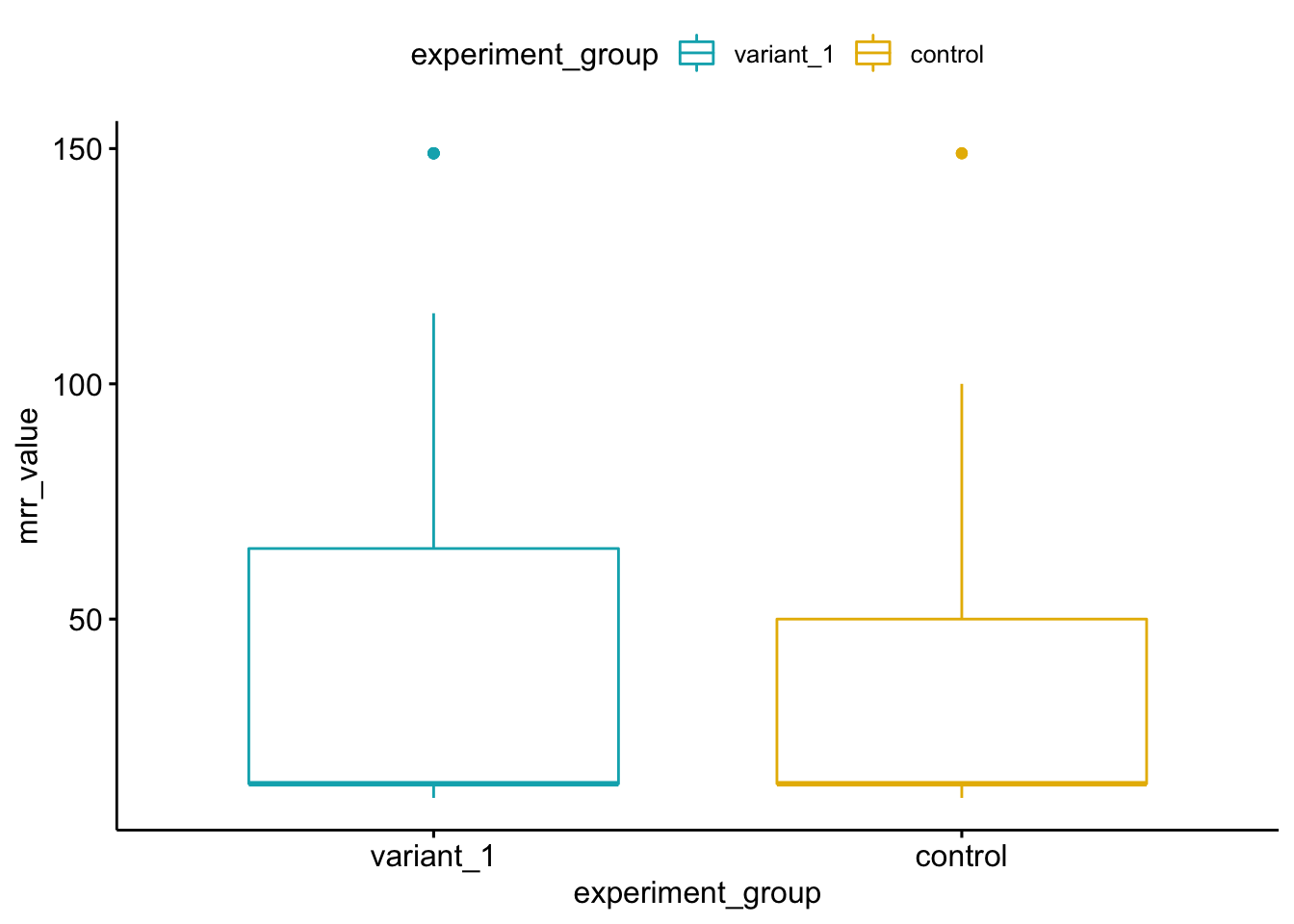
We can see in the above box plot graph that the variation group has more users with higher MRR values, which is increasing the MRR mean and resulting in a higher 75th percentile MRR value. We can dig into this just a little bit more by looking at the MRR amount by experiment group, visualized by density.
ggdensity(mrr, x = "mrr_value", add = "mean", rug = TRUE,
          color = "experiment_group", fill = "experiment_group", facet.by = "experiment_group", palette = c("#E7B800", "#00AFBB"),
          ylab = "Density", xlab = "MRR Amount")
## Warning: Removed 3391 rows containing non-finite values (stat_density).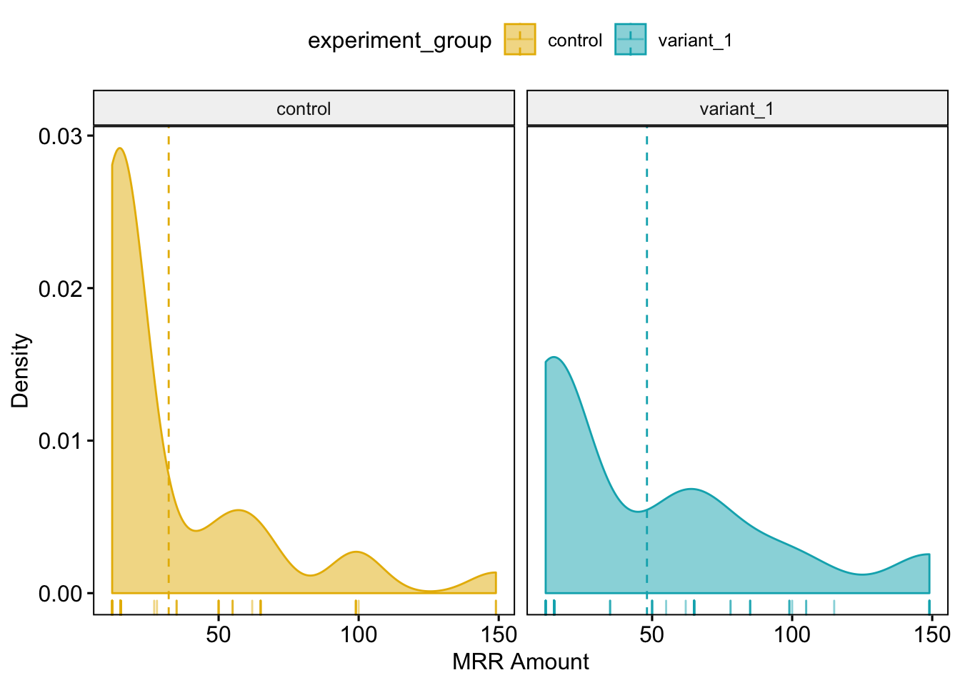
We can see that the two groups have different general shapes, with densities shifted much more to the right in the variation group. This makes sense given the additional 22 users on both Publish and Analyze paid subscriptions in the Variation group.
In order to test this change in density for statistical significance, we will look at the MRR per signup, which will account for differences in MRR where either more users purchased a lower price plan or fewer purchased at a higher priced plan. In order to do this, we will run a Mann Whitney Wilcoxon Test, which is a statistical hypothesis test that is the non-parametric equivalent to the t-test, and DOES NOT require data to be normally distributed.
The Null Hypothesis is that the difference between the two populations is zero (i.e. there is no difference.) The Alternative Hypothesis is that the difference between the two populations is not zero (i.e. there is a difference.)
result <- wilcox.test(mrr_value ~ experiment_group, data = mrr,
            conf.int = TRUE, conf.level = 0.95)
result
##
## Wilcoxon rank sum test with continuity correction
##
## data: mrr_value by experiment_group
## W = 3475, p-value = 0.01406
## alternative hypothesis: true location shift is not equal to 0
## 95 percent confidence interval:
## -3.000067e+00 -5.267197e-05
## sample estimates:
## difference in location
## -2.563398e-05With a p-value of 0.01406, the difference between the two experiment groups IS statistically significant, which indicates that the $15.98 greater MRR per paid user observed in the variant group has a little more than a 1 out of 100 chance of occurring from natural variance.
Bottom line, there is an observed 49% increase in MRR generated by the variation group, with the control generating $2993 and the variation generating $4479.
Let’s also take a per product view of MRR.
users3 <- users %>%
  mutate(mrr_value = subscription_revenue) %>%
  select(account_id, experiment_group, subscription_product, mrr_value)

mrr_by_product <- distinct(users3) %>%
  unite(group_and_product, c("experiment_group", "subscription_product")) %>%
  group_by(account_id, group_and_product) %>%
  summarise(mrr_value = sum(mrr_value))
summary_by_group <- mrr_by_product %>%
filter(!is.na(mrr_value)) %>%
group_by(group_and_product) %>%
summarise(
paid_users = sum(if_else(mrr_value > 0, 1, 0), na.rm = TRUE),
min_mrr = min(mrr_value, na.rm = TRUE),
max_mrr = max(mrr_value, na.rm = TRUE),
median_mrr = median(mrr_value, na.rm = TRUE),
mean_mrr = mean(mrr_value, na.rm = TRUE),
sum_mrr = sum(mrr_value, na.rm = TRUE),
std_dev_mrr = sd(mrr_value, na.rm = TRUE),
) %>%
gather(key = "key", value = "value", 2:8) %>%
spread(key = "group_and_product", value = "value") %>%
arrange(desc(key)) %>%
rename(metric = key) %>%
kable(digits = 2) %>%
kable_styling(bootstrap_options = c("striped", "hover", "condensed"))
summary_by_group| metric | control_analyze | control_publish | variant_1_analyze | variant_1_publish |
|---|---|---|---|---|
| sum_mrr | 683.00 | 2310.00 | 1705.00 | 2809.00 |
| std_dev_mrr | 7.84 | 26.57 | 4.26 | 29.44 |
| paid_users | 15.00 | 87.00 | 35.00 | 89.00 |
| min_mrr | 28.00 | 12.00 | 35.00 | 12.00 |
| median_mrr | 50.00 | 15.00 | 50.00 | 15.00 |
| mean_mrr | 45.53 | 26.55 | 48.71 | 31.56 |
| max_mrr | 50.00 | 99.00 | 50.00 | 99.00 |
We can see that the variant group generated more MRR and had more paying customers (as stated previously in this analysis) for each product, compared to the control group.
Let’s now look at a box plot for this per product MRR dataframe.
mrr_by_product_1 <- mrr_by_product %>%
  filter(!is.na(mrr_value))

ggboxplot(mrr_by_product_1, x = "group_and_product", y = "mrr_value",
          color = "group_and_product",
          ylab = "mrr_value", xlab = "group_and_product")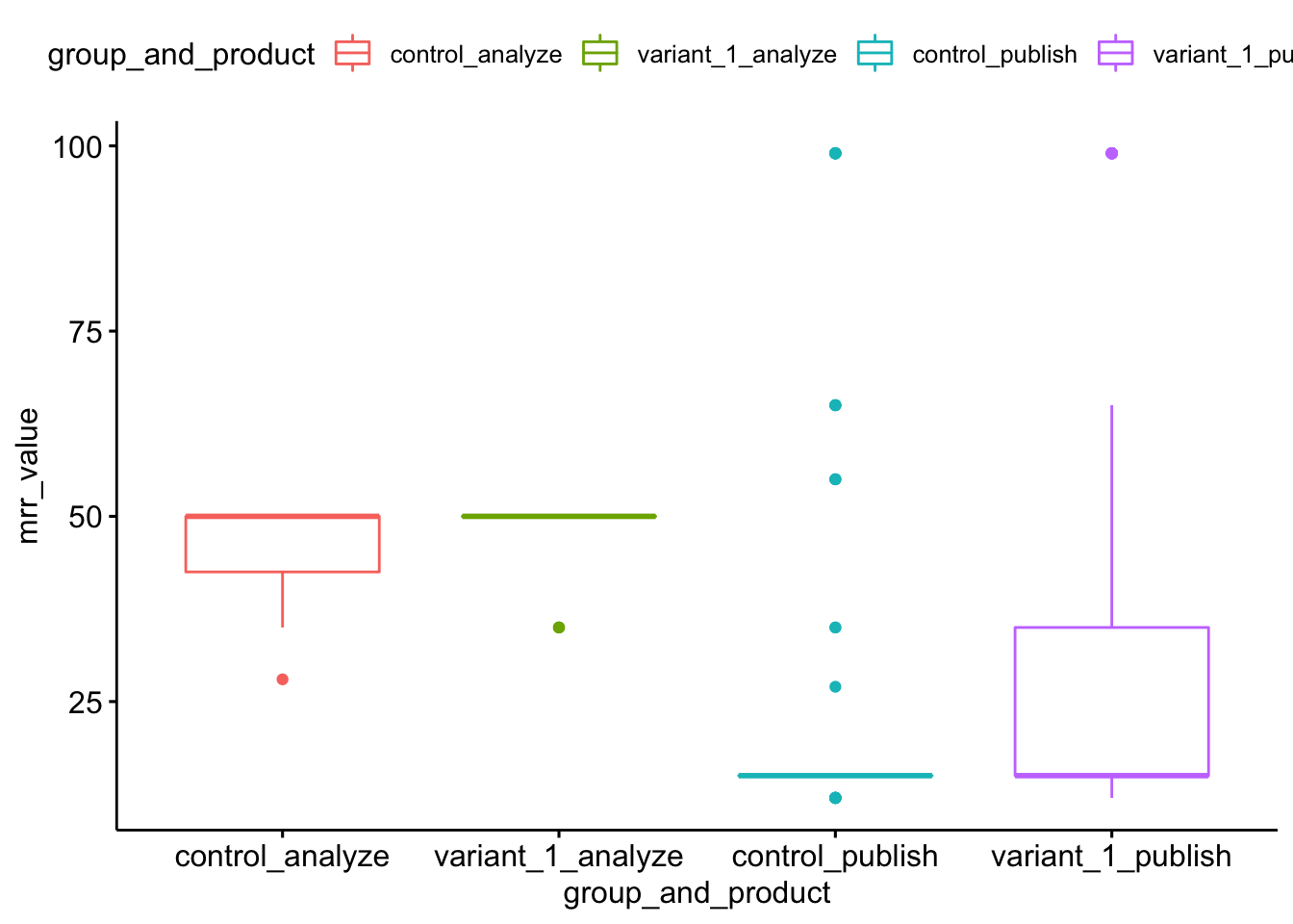
If you’ve made it this far in the analysis, you might also be interested in seeing the breakdown of MRR per plan, so as to see what kind of impact the variation treatment might have had on Publish business plan conversions, since this experiment did significantly change the experience of the /business page.
users3 <- users %>%
  mutate(mrr_value = subscription_revenue) %>%
  select(account_id, experiment_group, subscription_product, subscription_plan_id, mrr_value)

mrr_by_plan <- distinct(users3) %>%
  group_by(account_id, experiment_group, subscription_product, subscription_plan_id) %>%
  summarise(mrr_value = sum(mrr_value))
summary_by_plan <- mrr_by_plan %>%
filter(!is.na(mrr_value)) %>%
group_by(subscription_plan_id, subscription_product, experiment_group) %>%
summarise(
paid_users = sum(if_else(mrr_value > 0, 1, 0), na.rm = TRUE),
sum_mrr = sum(mrr_value, na.rm = TRUE),
) %>%
arrange(subscription_plan_id, desc(sum_mrr)) %>%
kable(digits = 2) %>%
kable_styling(bootstrap_options = c("striped", "hover", "condensed"))
summary_by_plan| subscription_plan_id | subscription_product | experiment_group | paid_users | sum_mrr |
|---|---|---|---|---|
| analyze_pro_y_336_201912 | analyze | control | 1 | 28 |
| analyze-no-early-access-discount-10-profiles | analyze | variant_1 | 32 | 1600 |
| analyze-no-early-access-discount-10-profiles | analyze | control | 11 | 550 |
| analyze-pro-8 | analyze | control | 3 | 105 |
| analyze-pro-8 | analyze | variant_1 | 3 | 105 |
| business_v2_small_monthly | publish | variant_1 | 11 | 1089 |
| business_v2_small_monthly | publish | control | 8 | 792 |
| premium_business_v1_monthly | publish | variant_1 | 6 | 390 |
| premium_business_v1_monthly | publish | control | 4 | 260 |
| premium_business_v1_yearly | publish | control | 3 | 165 |
| premium_business_v1_yearly | publish | variant_1 | 3 | 165 |
| pro_v1_monthly | publish | control | 57 | 855 |
| pro_v1_monthly | publish | variant_1 | 48 | 720 |
| pro_v1_yearly | publish | control | 14 | 168 |
| pro_v1_yearly | publish | variant_1 | 12 | 144 |
| publish_premium_m_35_201910 | publish | variant_1 | 7 | 245 |
| publish_premium_m_35_201910 | publish | control | 2 | 70 |
| publish_premium_y_336_201910 | publish | variant_1 | 2 | 56 |
Final Thoughts
Given the above observations, the result of the experiment is that there were favorable financial outcomes from the variation treatment changes made to the /business page. Though we did see a small drop in Publish trials started, there was a big increase in Analyze trials started. Even with this slight drop in Publish trials started, total number of users that converted to a Publish paid subscriptions increased slightly, as did the MRR those users generated. Additionally, the number of users that converted to a paid Analyze subscription increased significantly, as did the amount of MRR they generated. Total MRR generated by the variant group was $1486 more than the control group, which was a 49% increase.
We recommend enabling the Solutions V2 treatment changes for 100% of traffic.