DTC Publish Usage

Summary

• Most DTC users subscribe to the Pro and Premium plans.
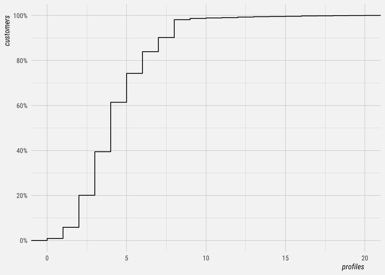
• Around 62% of paying DTC customers connect 4 or fewer profiles and around 75% connect 5 or fewer.
• Instagram and Facebook profiles are most commonly connected, and most DTC users tend to create posts for Instagram.
• DTC customers tend to have very few team members. Of those that do have access to team members (Premium and Business customers), around 95% have five or fewer. Around 45% of eligible customers have no team members.
• Of active DTC customers, most create updates on 2 or 3 days of a given (active) week. There is a long tail of users that are active on more days of the week.
• For Pro customers, post analytics and calendar are the most commonly used features. For Premium and up customers, it’s post analytics, stories, hashtag groups, and the calendar.
• Around 27% of customers schedule posts to go out within a day, on average. Over 80% of customers schedule posts to go out within a week, on average.

Which Plans do DTC Customers Have

The motivation is to see if there is a single plan that stands out to users. We’ll collect the data we need with the SQL query below.

# connect to bigquery
con <- dbConnect(
  bigrquery::bigquery(),
  project = "buffer-data"
)

# define sql query
sql <- "
  select 
    u.id as user_id
    , u.billing_plan
    , u.account_id
    , i.company_size
    , i.company_type
    , i.company_market
    , max(t.timestamp) as last_action_at
    , count(distinct p.id) as profiles
    , count(distinct 
              case when p.service = 'twitter' 
              then p.id else null end) as twitter_profiles
    , count(distinct 
              case when p.service = 'instagram' 
              then p.id else null end) as ig_profiles
    , count(distinct 
              case when p.service = 'instagram' and service_type = 'business' 
              then p.id else null end) as ig_biz_profiles
    , count(distinct 
              case when p.service = 'facebook' 
              then p.id else null end) as fb_profiles
    , count(distinct 
              case when p.service = 'pinterest' 
              then p.id else null end) as pinterest_profiles
    , count(distinct 
              case when p.service = 'linkedin' 
              then p.id else null end) as linkedin_profiles
  from dbt_buffer.publish_users u
  inner join dbt_buffer.segment_identifies i
    on u.account_id = i.user_id
    and i.company_type = 'online-store'
  left join dbt_buffer.segment_tracks t
    on t.user_id = u.account_id
  left join dbt_buffer.publish_profiles p
    on u.id = p.user_id
    and (not p.is_disabled or p.is_disabled is null)
    and (not p.is_deleted or p.is_deleted is null)
  where u.created_at >= '2019-06-01'
  group by 1,2,3,4,5,6
"
  
# query BQ
dtc <- dbGetQuery(con, sql)

# save data
saveRDS(dtc, "dtc_plans.rds")

The plots below show the number of DTC users by plan. The Pro plan is the most common by far for paying customers.

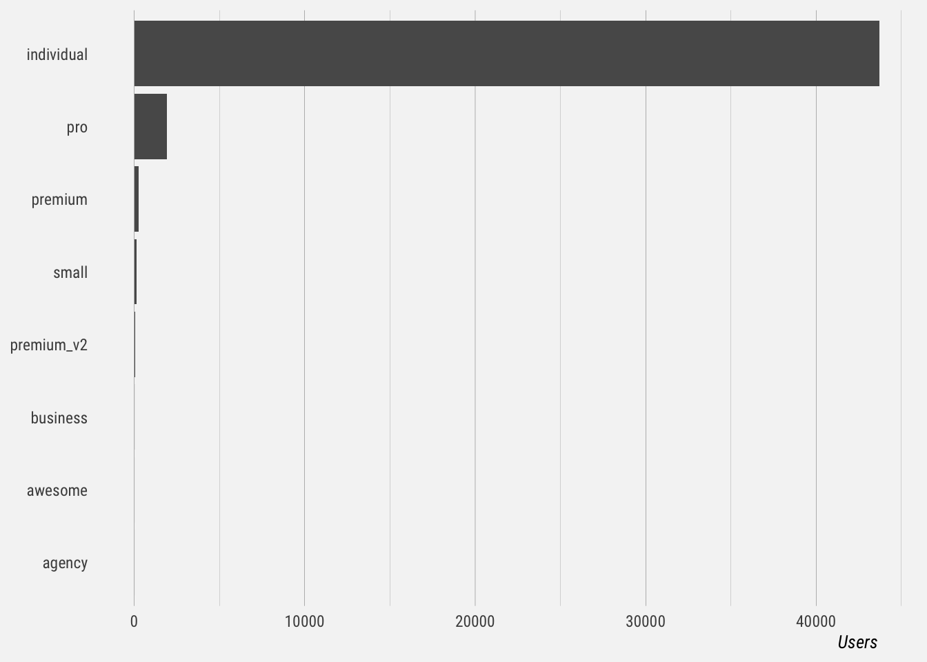
Around 5% of DTCs that sign up for Publish are paying customers.

# count paid
dtc %>% 
  group_by(paid = billing_plan != "individual") %>% 
  summarise(users = n_distinct(user_id)) %>% 
  mutate(prop = percent(users / sum(users)))

## `summarise()` ungrouping output (override with `.groups` argument)

## # A tibble: 2 x 3
##   paid  users prop 
##   <lgl> <int> <chr>
## 1 FALSE 43659 95%  
## 2 TRUE   2352 5%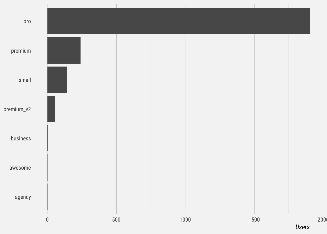

Now let’s see how many are “active”. If the user’s last action occurred in the past 30 days we’ll consider them active. Around 30% of DTC users that have signed up since June 2019 are currently active.

# count active
dtc %>% 
  group_by(active = as.Date(last_action_at) >= "2020-04-13") %>% 
  summarise(users = n_distinct(user_id)) %>% 
  mutate(prop = percent(users / sum(users)))

## `summarise()` ungrouping output (override with `.groups` argument)

## # A tibble: 2 x 3
##   active users prop 
##   <lgl>  <int> <chr>
## 1 FALSE  32784 71%  
## 2 TRUE   13227 29%

How Many Channels do DTCs Connect

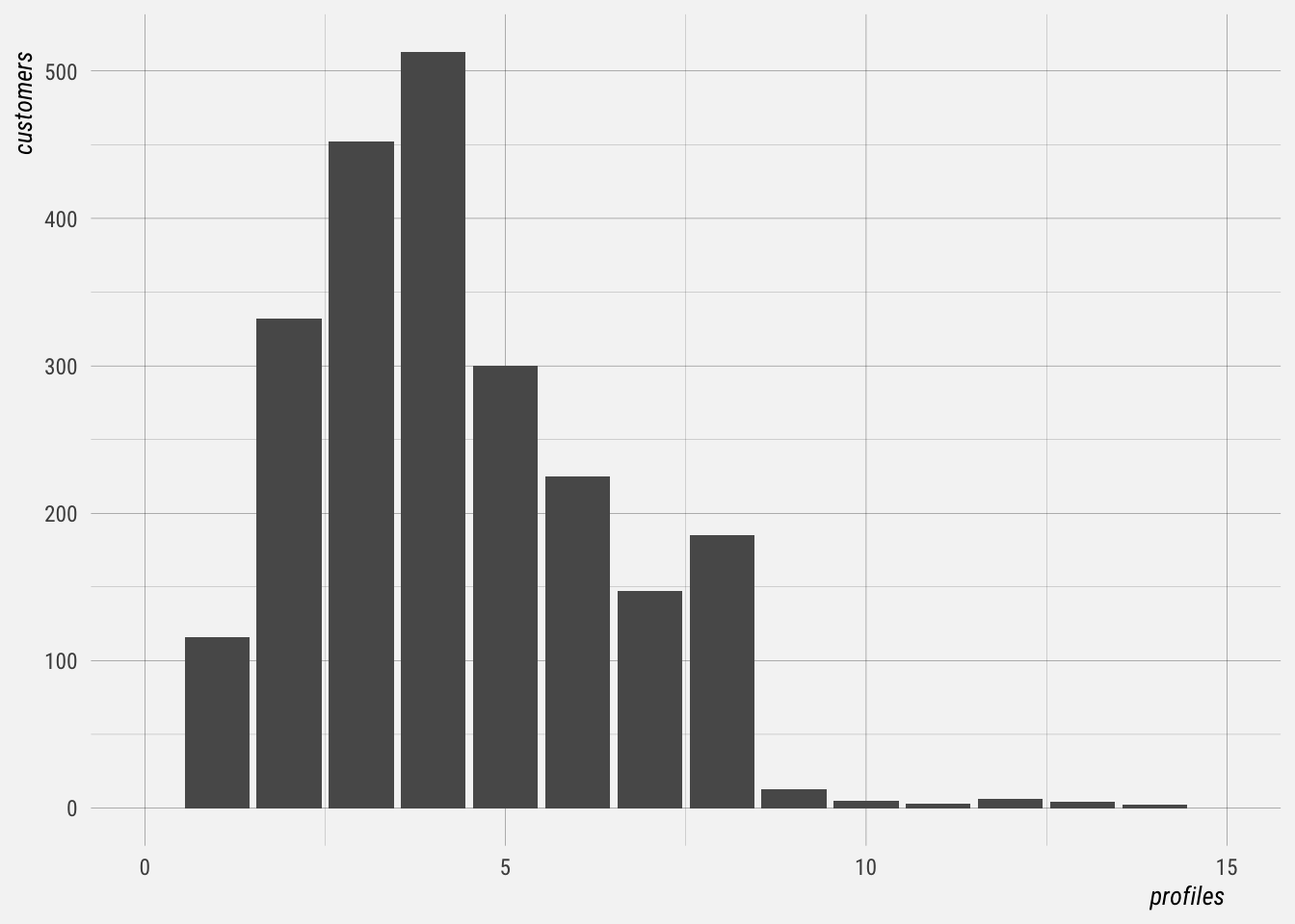
We’ll exclude free users from the plots of this distribution. The plots show that most DTC customers (~62%) connect 4 or fewer profiles. Around 75% of DTC customers have 5 or fewer profiles, and around 98% have 8 or fewer profiles.

What Types of Channels Are Connected?

We’ll plot the proportion of DTC customers that have at least one profile from each social network. Unsurprisingly Facebook and Instagram are the most common profile types, followed by Twitter, Linkedin, and Pinterest.

## `summarise()` regrouping output by 'channel' (override with `.groups` argument)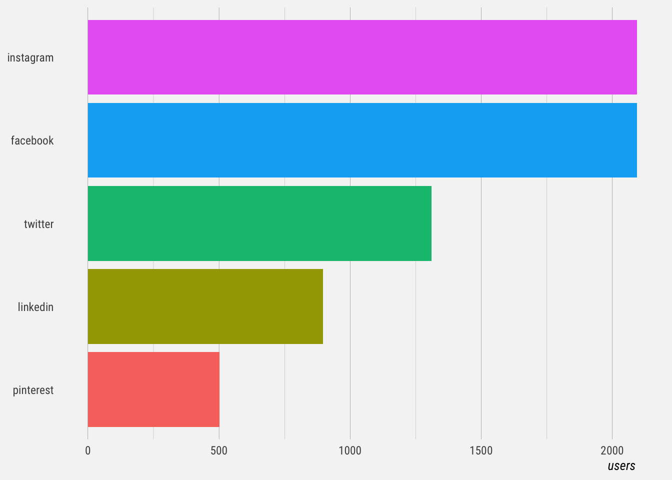

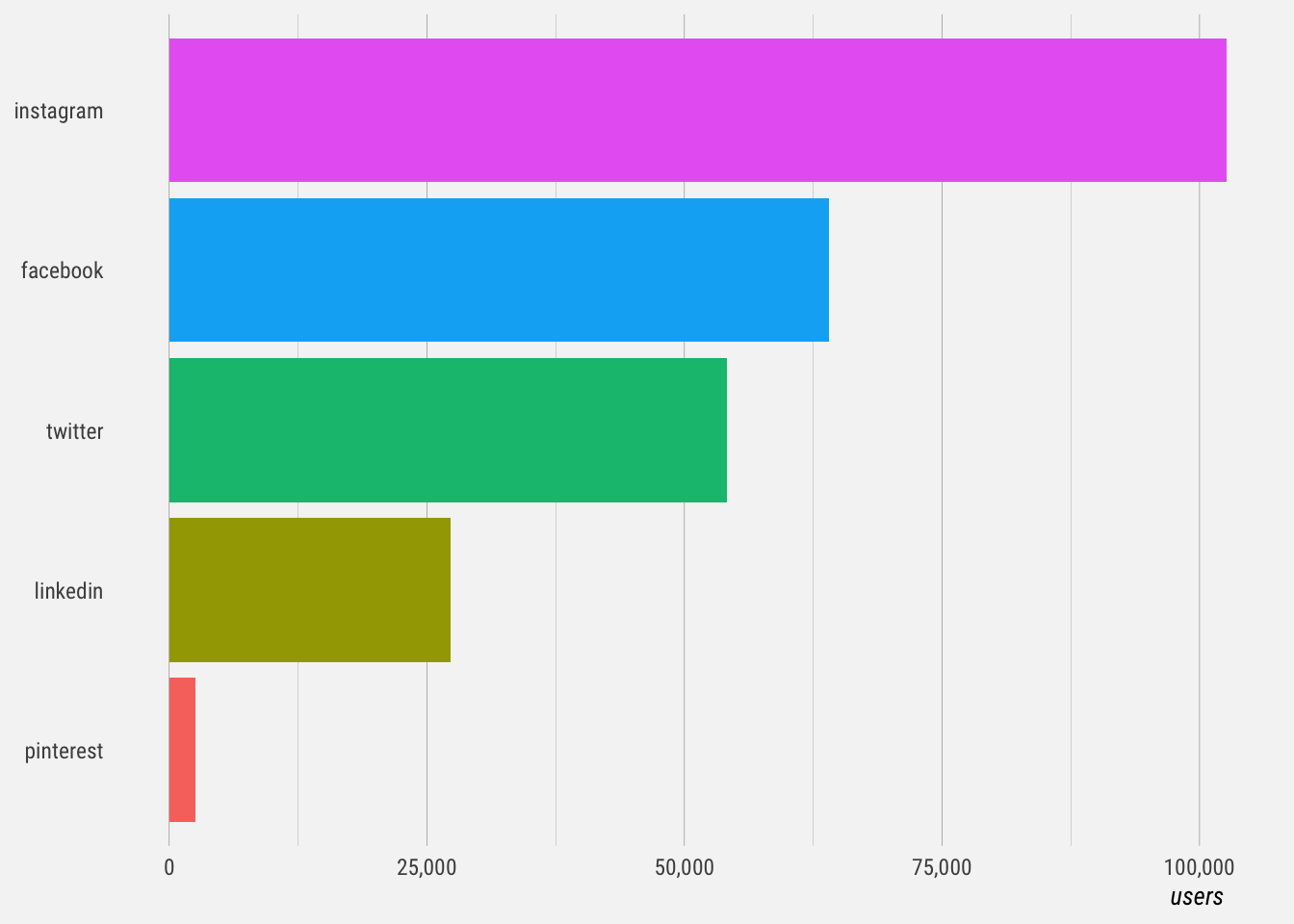
What Channels do DTCs Share to?

We’ll only look at users that have shared updates in the past 90 days. The plot includes users on the free plan. It shows that most DTC users share posts to Instagram, followed by Facebook, Twitter, Linkedin, and Pinterest.

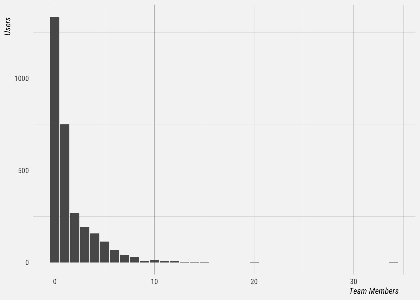
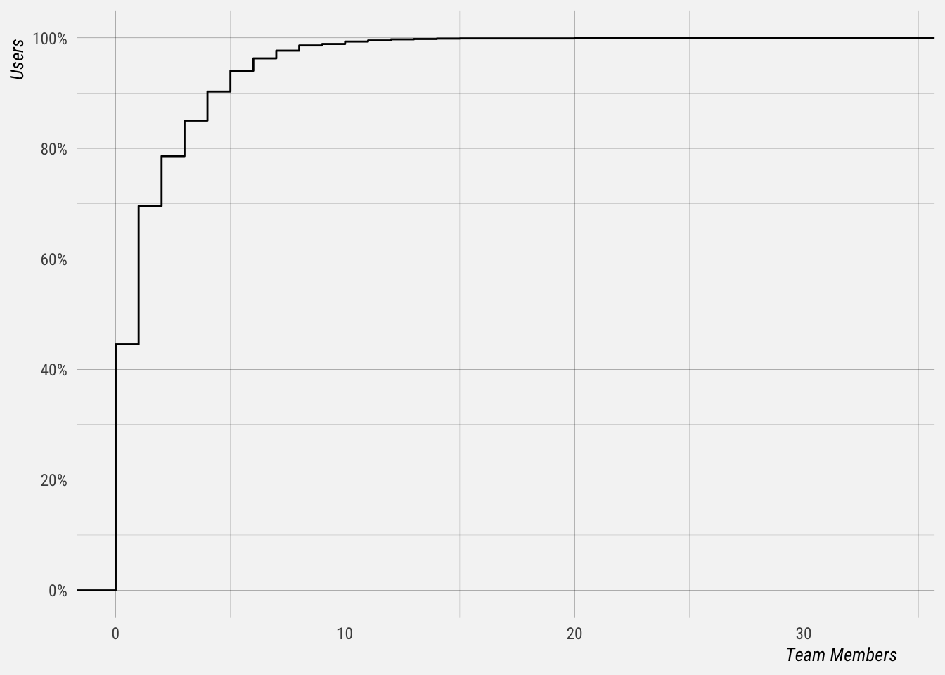
How Many Team Members do DTCs Have?

We’ll exclude users on the free plan and users on the Pro plan from the plots below because they can’t have team members. Most DTC customers have relatively few team members:

• Around 45% have no team members
• Around 69% have 1 or 0 team members
• Around 95% have 5 or fewer team members

How Often do DTCs Post?

# connect to bigquery
con <- dbConnect(
  bigrquery::bigquery(),
  project = "buffer-data"
)

# define sql query
sql <- "
  select
    u.id as user_id
    , u.billing_plan
    , date(up.created_at) as post_date
    , count(distinct up.id) as posts
  from dbt_buffer.publish_users u
  inner join dbt_buffer.segment_identifies i
    on u.account_id = i.user_id
    and i.company_type = 'online-store'
  left join dbt_buffer.publish_profiles p
    on p.user_id = u.id
  left join dbt_buffer.publish_updates up
    on p.id = up.profile_id
    and up.status not in ('service', 'service_reply')
    and up.created_at >= '2019-06-01'
  where u.created_at >= '2019-06-01'
  group by 1,2,3
"
  
# query bigquery
posts <- dbGetQuery(con, sql)

# save data
saveRDS(posts, "dtc_posts.rds")

For users that do share posts, we’ll summarise the number of posts they share per week as well as the number of days per week that they create posts. We’ll only include users that created updates in two separate weeks.

# summarise by week
by_user <- posts %>% 
  group_by(user_id, billing_plan, week) %>% 
  summarise(days = n_distinct(post_date),
            posts = sum(posts)) %>% 
  group_by(user_id, billing_plan) %>% 
  summarise(weeks = n_distinct(week),
            avg_days = mean(days, na.rm = TRUE),
            avg_posts = mean(posts, na.rm = TRUE)) %>% 
  filter(weeks >= 2)

## `summarise()` regrouping output by 'user_id', 'billing_plan' (override with `.groups` argument)

## `summarise()` regrouping output by 'user_id' (override with `.groups` argument)

# plot distribution of avg days with posts
by_user %>% 
  filter(billing_plan != "agency") %>% 
  ggplot(aes(x = avg_days, color = billing_plan)) +
  geom_density() +
  facet_wrap(~billing_plan, scales = "free_y") +
  labs(x = "Average Days with Posts Created",
       y = "Density",
       title = "Distribution of Mean Posting Days Per Week",
       subtitle = "DTC Users with Two Weeks of Posting Data") +
  scale_x_continuous(breaks = seq(0, 7, 1)) +
  theme(legend.position = "none")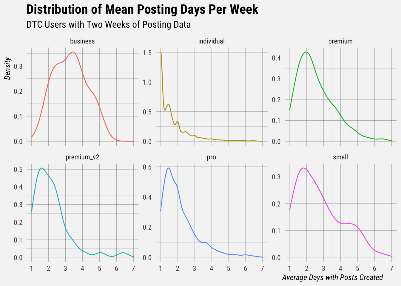

These plots suggest that it’s most common for active DTC users to create posts on one or two days per week. Users on business plans are more likely to spend more days of the week creating posts. Each distribution has a long tail, which means that there is a significant proportion of users that creates posts on more than two days per week. This is shown more clearly in the plots of the cumulative distribution functions (CDFs) below.

# plot distribution of avg days with posts
by_user %>% 
  filter(billing_plan != "agency") %>% 
  ggplot(aes(x = avg_days, color = billing_plan)) +
  stat_ecdf() +
  facet_wrap(~billing_plan) +
  labs(x = "Average Days with Posts Created",
       y = NULL,
       title = "CDF of Posting Days Per Week",
       subtitle = "DTC Users with Two Weeks of Posting Data") +
  scale_x_continuous(breaks = seq(0, 7, 1)) +
  scale_y_continuous(breaks = seq(0, 1, 0.2), labels = percent) +
  theme(legend.position = "none")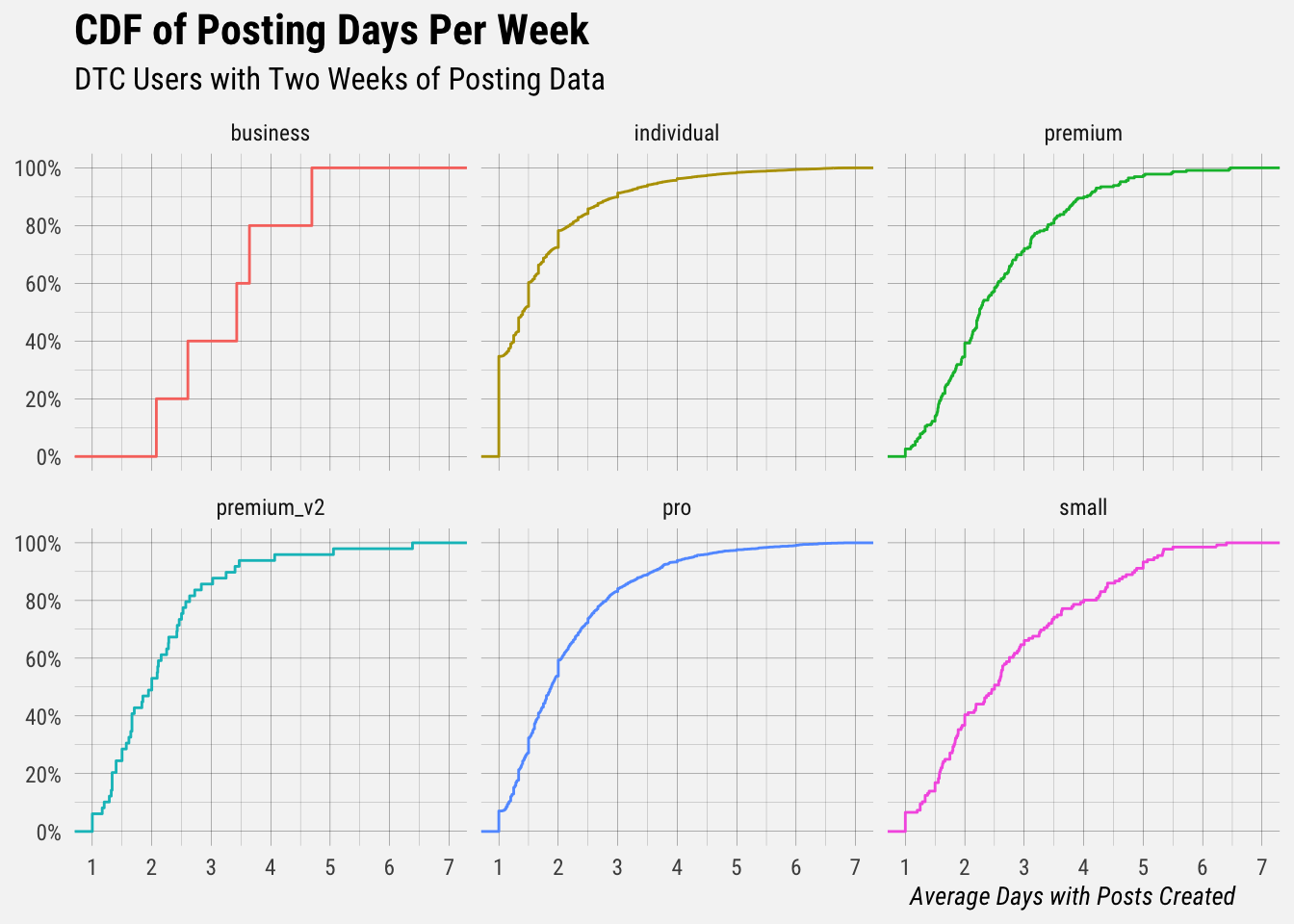

Around 60% of active Pro DTC customers create posts on two or fewer days per week. This suggests that around 40% create posts on three or more days per week.

Around 40% of active Premium and Small Business DTC customers create posts on two or fewer days per week. This suggests that around 60% create posts on three or more days per week.

It’s important to remember that these distributions only include active customers that have created posts in at least two separate weeks. It excludes weeks in which users don’t create any posts.

How Far Out Are They Planning?

We’ll take a random sample of updates from DTC customers and try to estimate this. We’ll also only look at paying customers.

# connect to bigquery
con <- dbConnect(
  bigrquery::bigquery(),
  project = "buffer-data"
)

# define sql query
sql <- "
  select distinct
    up.created_at as update_date
    , up.due_at as due_date
    , up.profile_service
    , up.id as update_id
    , u.id as user_id
    , u.billing_plan
    , rand() as random
  from dbt_buffer.publish_users u
  inner join dbt_buffer.segment_identifies i
    on u.account_id = i.user_id
    and i.company_type = 'online-store'
  left join dbt_buffer.publish_profiles p
    on p.user_id = u.id
  left join dbt_buffer.publish_updates up
    on p.id = up.profile_id
    and up.status not in ('service', 'service_reply')
    and up.created_at >= '2019-06-01'
  where u.created_at >= '2019-06-01'
  and u.billing_plan != 'individual'
  order by random
  limit 500000
"
  
# query bigquery
post_dates <- dbGetQuery(con, sql)

# save data
saveRDS(post_dates, "dtc_post_dates.rds")

For this random sample of 500 thousand updates, let’s plot the distribution of the number of days between the date the post was created and the date it was due.

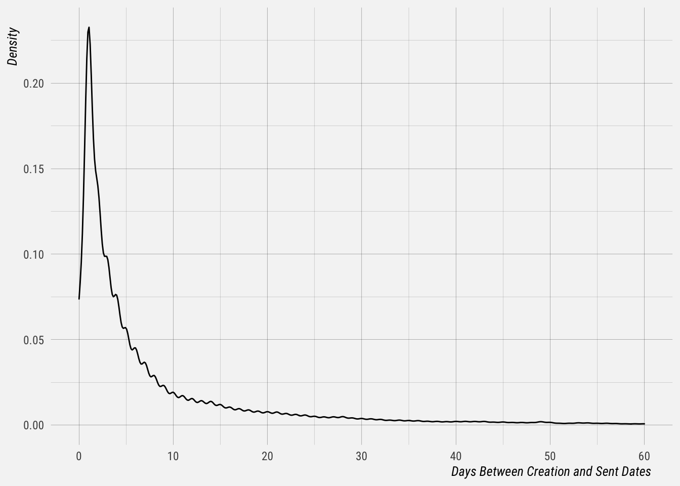
We can see that it’s most common for posts to be scheduled to go out in the very near future. Of this random sample of 500 thousand updates, around 30% were scheduled to go out within one day. Over 50% were scheduled to go out within two days, and over 70% were scheduled to go out within one week.

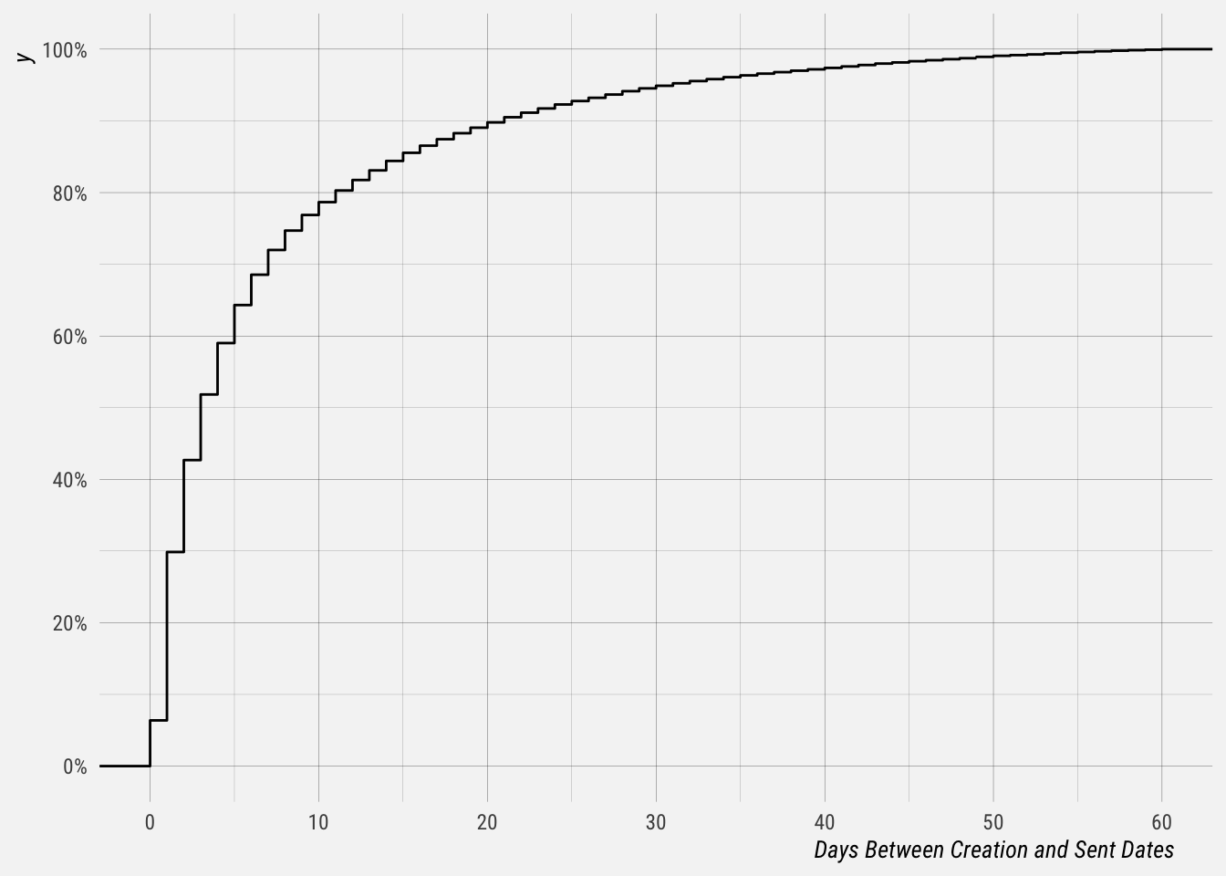
This could be skewed by prolific users, so let’s do some further summarization. For each user we’ll calculate the median number of days between the date the post was created and the date it was supposed to be sent out.

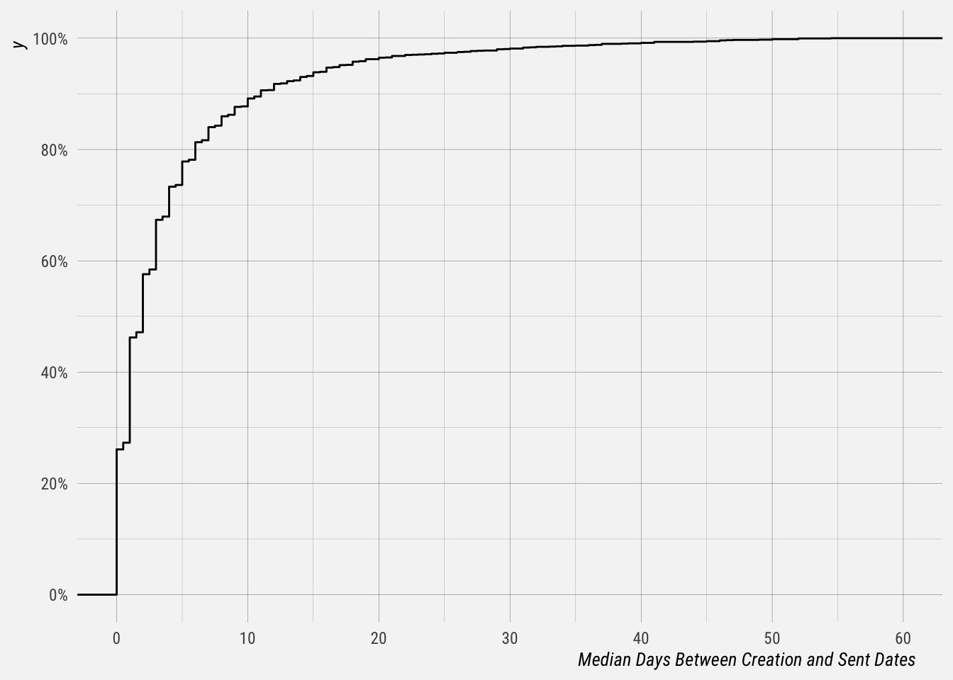
This is more informative. Around 27% of customers schedule posts to go out within a day, on average. Over 80% of customers schedule posts to go out within a week, on average.

Which Features Are Used Most?

We’ll collect the relevant data from BigQuery with the SQL query below. At the time this analysis was written, the Campaigns feature was still relatively new. Because of this, I’ve decided to exclude it from the features analyzed.

# connect to bigquery
con <- dbConnect(
  bigrquery::bigquery(),
  project = "buffer-data"
)

# define sql query
sql <- "
  select 
    u.id as user_id
    , u.billing_plan
    , max(t.timestamp) as last_action_at
    , count(distinct
              case when pv.name = 'analytics posts' 
              then pv.id else null end) as post_analytics_views
    , count(distinct
              case when pv.name = 'analytics overview' 
              then pv.id else null end) as overviews_analytics_views
    , count(distinct
              case when t.event = 'shop_grid_link_added' 
              then t.id else null end) as shop_grid_links_added
    , count(distinct
              case when t.event = 'story_group_created' 
              then t.id else null end) as story_groups_created
    , count(distinct
              case when t.event = 'draft_submitted' 
              then t.id else null end) as drafts_submitted
    , count(distinct
              case when t.event = 'hashtag_group_created' 
              then t.id else null end) as hashtag_groups_created
    , count(distinct c.id) as calendar_views
  from dbt_buffer.publish_users u
  inner join dbt_buffer.segment_identifies i
    on u.account_id = i.user_id
    and i.company_type = 'online-store'
  left join dbt_buffer.segment_tracks t
    on t.user_id = u.account_id
  left join segment_publish.page_viewed_view pv
    on u.account_id = pv.user_id
    and pv.name in ('analytics posts', 'analytics overview')
    and pv.original_timestamp >= '2019-06-01'
  left join segment_publish_classic.pages_view c
    on c.user_id = u.account_id
    and c.name = 'Publish Classic Calendar'
    and c.original_timestamp >= '2019-06-01'
  where u.created_at >= '2019-06-01'
  group by 1,2
"
  
# query BQ
features <- dbGetQuery(con, sql)

# save users
saveRDS(features, "dtc_features.rds")

## `summarise()` ungrouping output (override with `.groups` argument)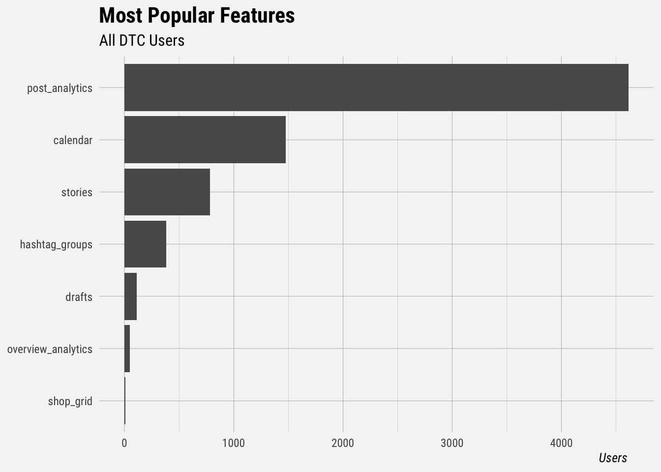

This plot shows that post analytics, calendar, and stories are the features used by the most users. This is influenced by the plans users are on though, so it would be useful to create this plot for each plan.

## `summarise()` regrouping output by 'feature' (override with `.groups` argument)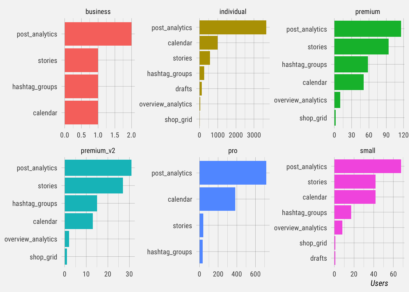

For Pro customers, post analytics and calendar are the most commonly used features. For Premium and up customers, it’s post analytics, stories, hashtag groups, and the calendar.