Updated on February 1, 2021.
In this analysis we will attempt to estimate the effect that using the engagement feature has on retention for Buffer customers.
The dataset used contains around 38 thousand Buffer customers that started subscriptions on or after January 2020. We’ll separate the customers into groups defined by whether or not they replied to a comment during the period in which their subscriptions were active.
Key Findings
The data suggests that customers that replied to a comment with the engagement feature churn at significantly lower rates than those that did not.
This outcome is likely affected by selection bias – customers that used the feature likely have Instagram accounts with more followers and engagement, which would have granted them earlier access to the product. Customers that churned were less likely to have been invited to use Engage.
The data could suggest that using the engagement feature lowers the likelihood of churning, or that active customers with low churn probabilities are more likely to make use of the feature.
Data Exploration
Around 5% of customers in our dataset replied to a comment with the engagement feature.
# count engage users
users %>%
  count(used_engage) %>%
  mutate(prop = percent(n / sum(n)))
## # A tibble: 2 x 3
## used_engage n prop
## <lgl> <int> <chr>
## 1 FALSE 36677 95%
## 2 TRUE 1878 5%Of customers that didn’t reply to a comment, around 35% have canceled their subscription. Only around 7% of customers that did reply to a commend have canceled. This stat shows that the data is potentially unbalanced or biased.
# count churned users
users %>%
  group_by(used_engage, canceled) %>%
  summarise(customers = n_distinct(stripe_customer_id)) %>%
  mutate(prop = customers / sum(customers))
## # A tibble: 4 x 4
## # Groups: used_engage [2]
## used_engage canceled customers prop
## <lgl> <lgl> <int> <dbl>
## 1 FALSE FALSE 23323 0.647
## 2 FALSE TRUE 12737 0.353
## 3 TRUE FALSE 1749 0.933
## 4 TRUE TRUE 126 0.0672To analyze the potential effect on retention we’ll use a common technique called survival analysis.
Survival Analysis
Survival analysis is a common branch of statistics used for analyzing the expected duration of time before a certain event occurs. It is commonly used in the medical field to analyze mortality rates, hence the term “survival”.
It’s especially useful when the data is right-censored, meaning there are cases in which the event hasn’t happened yet, but will likely happen at some time in the future. In the figures below, see the numbers with a “+”. These refer to customers that haven’t churned yet – their time to churn is X days “+”.
# build survival object
km <- Surv(users$time_to_cancel, users$canceled)

# preview data
head(km, 10)
## [1] 17+ 56+ 301+ 89+ 91+ 306+ 64+ 336+ 199+ 40+To begin our analysis, we use the formula Surv(time, canceled) ~ 1 and the survfit() function to produce the Kaplan-Meier estimates of the probability of “survival” over time. The times parameter of the summary() function gives some control over which times to print. Here we set it to print the estimates for 1, 30, 60 and 90 days, and then every 90 days thereafter.
# get survival probabilities
km_fit <- survfit(Surv(time_to_cancel, canceled) ~ 1, data = users)

# summarise
summary(km_fit, times = c(1, 7, 14, 30, 60, 90 * (1:10)))
## Call: survfit(formula = Surv(time_to_cancel, canceled) ~ 1, data = users)
##
## time n.risk n.event survival std.err lower 95% CI upper 95% CI
## 1 38309 383 0.990 0.000505 0.989 0.991
## 7 37301 312 0.982 0.000680 0.981 0.983
## 14 36450 150 0.978 0.000751 0.976 0.979
## 30 34531 1367 0.940 0.001240 0.937 0.942
## 60 28760 2943 0.855 0.001866 0.852 0.859
## 90 24170 2135 0.790 0.002200 0.785 0.794
## 180 14169 3772 0.651 0.002750 0.646 0.657
## 270 7219 1559 0.565 0.003165 0.558 0.571
## 360 2076 593 0.500 0.003850 0.492 0.507The survival column shows the estimate for the percentage of customers still active after a certain number of days after subscribing. For example, around 94% of subscriptions are still active by day 30 and around 85% are still active by day 60.
This curve can be plotted.
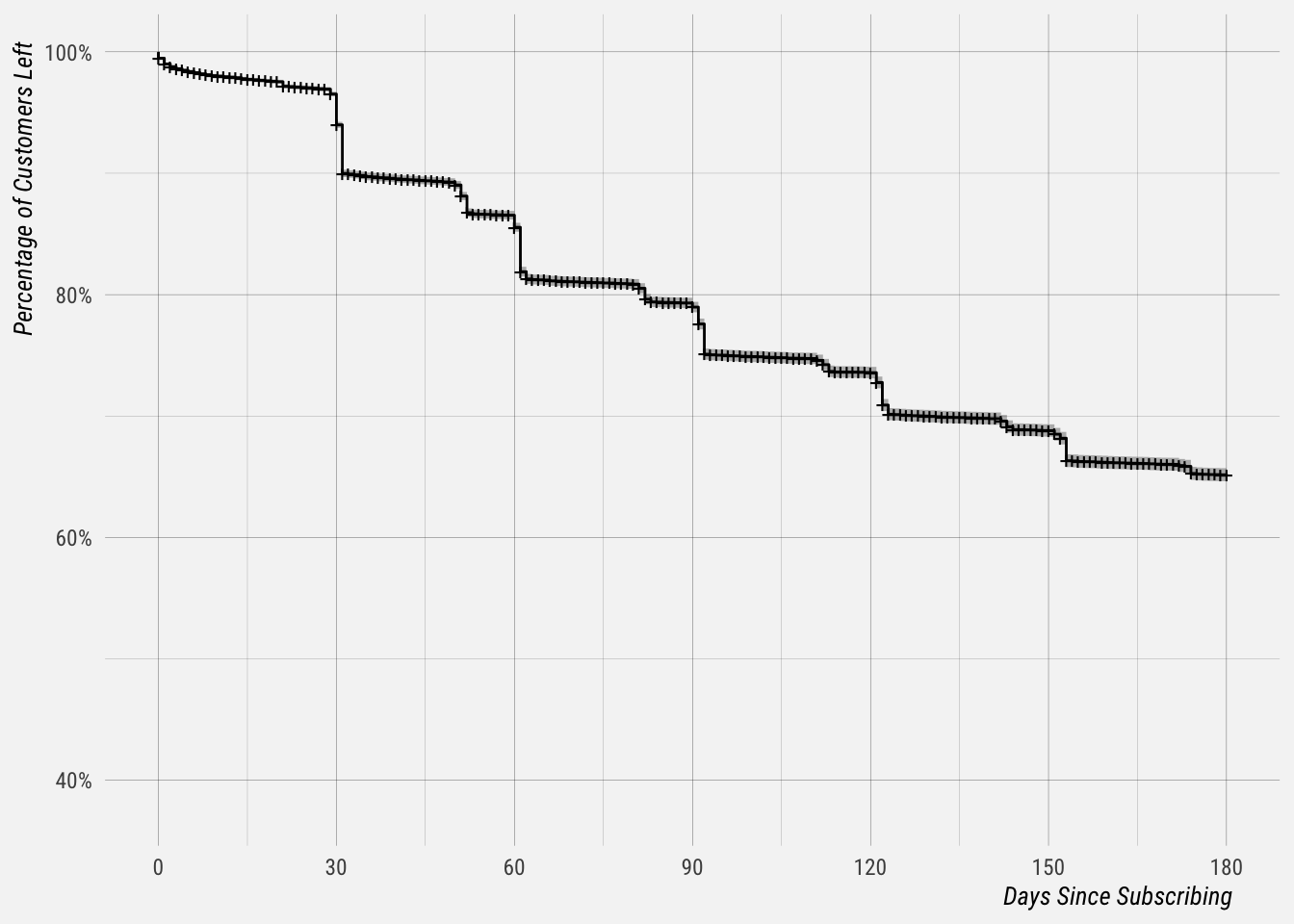
You can see dips in the curve every 30 days, which makes intuitive sense given monthly billing periods. Now lets segment the customers by whether or not they replied to a comment and fit survival curves for each group
# get survival probabilities for each segment
km_fit <- survfit(Surv(time_to_cancel, canceled) ~ used_engage, data = users)

# summarise
summary(km_fit, times = c(1, 7, 14, 30, 60, 90, 180))
## Call: survfit(formula = Surv(time_to_cancel, canceled) ~ used_engage,
## data = users)
##
## used_engage=FALSE
## time n.risk n.event survival std.err lower 95% CI upper 95% CI
## 1 36433 383 0.990 0.000531 0.989 0.991
## 7 35463 312 0.981 0.000714 0.980 0.982
## 14 34667 150 0.977 0.000789 0.975 0.978
## 30 32835 1362 0.937 0.001299 0.934 0.940
## 60 27205 2934 0.849 0.001949 0.845 0.853
## 90 22725 2121 0.780 0.002292 0.776 0.785
## 180 13252 3719 0.637 0.002843 0.632 0.643
##
## used_engage=TRUE
## time n.risk n.event survival std.err lower 95% CI upper 95% CI
## 1 1876 0 1.000 0.00000 1.000 1.000
## 7 1838 0 1.000 0.00000 1.000 1.000
## 14 1783 0 1.000 0.00000 1.000 1.000
## 30 1696 5 0.997 0.00130 0.995 1.000
## 60 1555 9 0.992 0.00224 0.987 0.996
## 90 1445 14 0.982 0.00330 0.976 0.989
## 180 917 53 0.940 0.00653 0.928 0.953We can see that, although the sample is small, customers that used Engage have churned at significantly lower rates than those that did not. For example, around 85% of customers that did not use Engage were still active by day 60, compared to around 99% of customers that did use Engage.
The survival curves show a seemingly huge difference in churn rates.
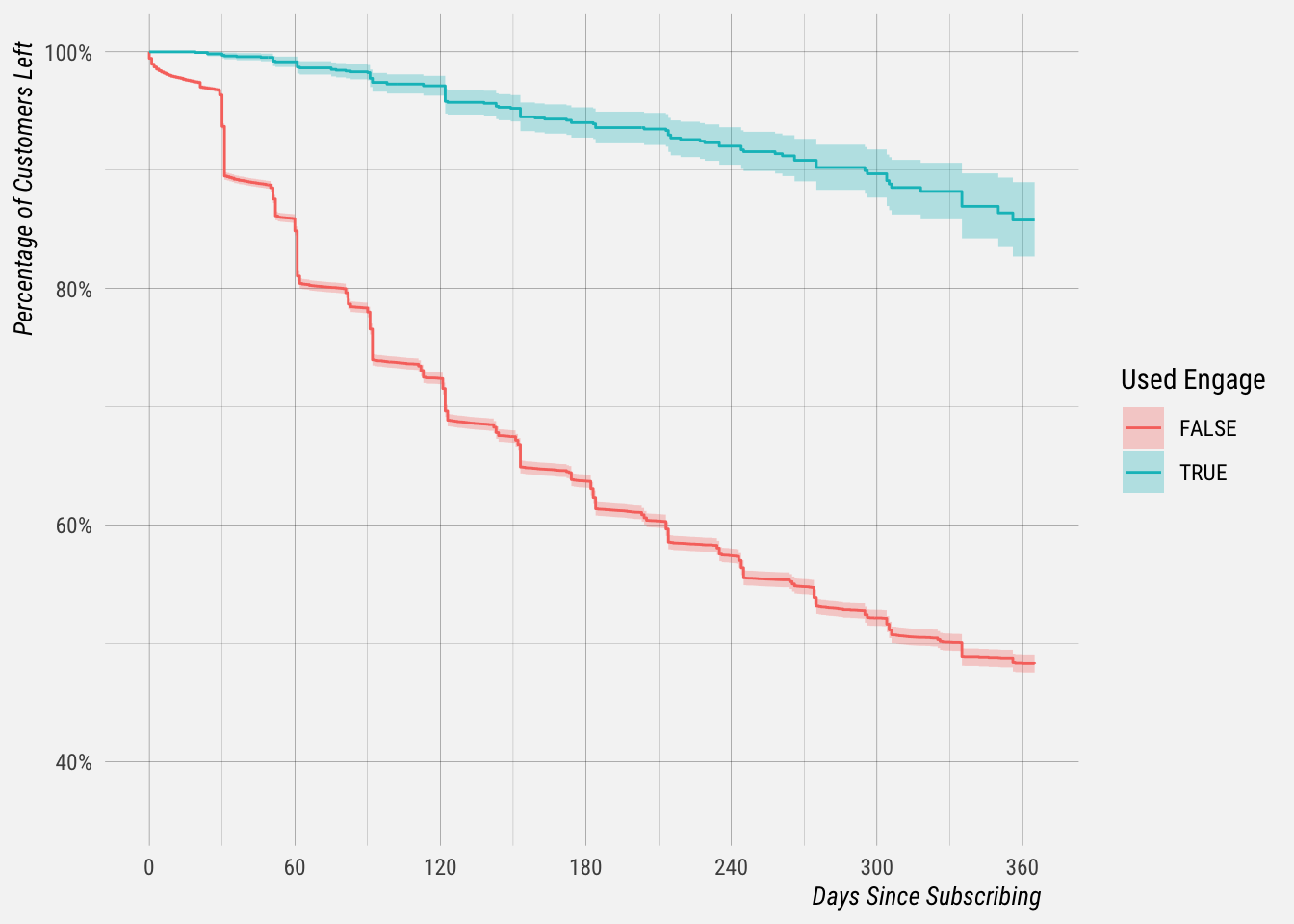
One should keep in mind that this is likely affected by bias in the data and causality has not been established.
Customers that replied to a comment in Engage were either part of a hand-selected batch of Business customers that had early access or self selected by replying to a comment on their own. The fact is that active customers were more likely to use the engagement feature and customers that churned were less likely to have had the opportunity to use it.
Pro Plans
We can segment the data further and see if the survival curves differ for Pro and Premium/Business subscriptions. The plot below shows that churn rates are significantly lower for both Pro and non-Pro subscriptions that have used Engage.
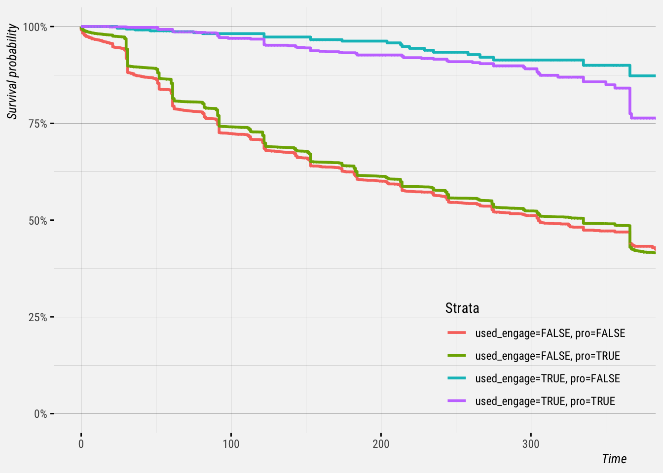
It’s worth mentioning again that causality hasn’t been established. People that have replied to a comment in Engage have been less likely to churn, but that doesn’t mean that the introduction of the engagement feature made them less likely to churn. It is more likely that these users were already more likely to be retained.