A Text Analysis of Churn Surveys

Data Tidying

In order to analyze the text efficiently, we’ll want to make use of some “tidy” data principles. To consider this data set tidy we need to have one token (or one observation in most other analyses) per row. A token in this text analysis is one word or a group of words.

To do this, we use the unnest_tokens() function in the tidytext package. This breaks the churn survey responses into individual words and includes one word per row while retaining the attributes (product, user_id, etc) of that word.

# unnnest the tokens
text_df <- users %>%
  unnest_tokens(word, details)

# glimpse data
glimpse(text_df)

## Rows: 56,488
## Columns: 9
## $ id        <chr> "30e7b498-57c9-4de4-8605-58b54ac0303d", "fab90ac9-ca7d-4a8b…
## $ user_id   <chr> "5e91ba841e1874251357e4bf", "5ca1d529fd16da3982477446", "5c…
## $ reason    <chr> "extenuating-circumstances", "not-using-anymore", "not-usin…
## $ timestamp <dttm> 2020-07-01 13:33:47, 2020-07-01 15:03:24, 2020-07-01 15:03…
## $ product   <chr> "publish", "publish", "publish", "publish", "publish", "pub…
## $ date      <date> 2020-07-01, 2020-07-01, 2020-07-01, 2020-07-01, 2020-07-01…
## $ month     <date> 2020-07-01, 2020-07-01, 2020-07-01, 2020-07-01, 2020-07-01…
## $ week      <date> 2020-06-28, 2020-06-28, 2020-06-28, 2020-06-28, 2020-06-28…
## $ word      <chr> "gracias", "please", "cancel", "and", "refund", "my", "102"…

Next we’ll remove stop words like “a”, “the”, etc. that aren’t useful to us.

# get stop words
data(stop_words)

# remove stop words from dataset
text_df <- text_df %>%
  anti_join(stop_words, by = "word")

Data Exploration

Now that the data has been restructured into a tidy format, we can do some exploration. Let’s start by looking at the most common terms present in the survey responses.

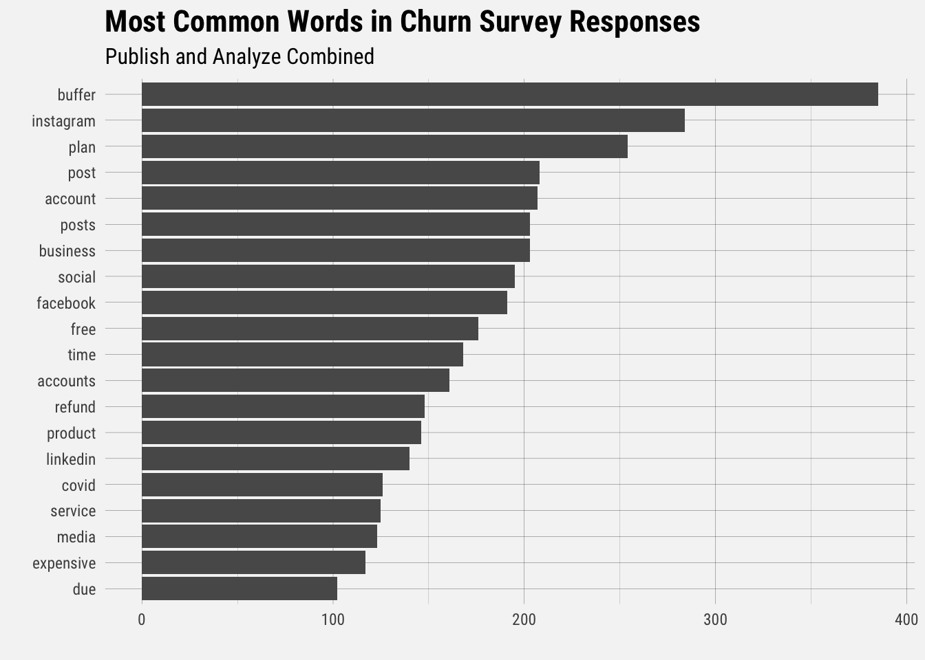
Unsurprisingly, “buffer” is the most common term. The terms “instagram” and “plan” follow, which suggests that users are still experiencing issues with Instagram and perhaps billing.

Next let’s look at words that occure with more frequency in Publish churn surveys compared to Analyze surveys.

To find these words, we can calculate the relative frequency of words that appear in the Publish churn survey and compare that to the relative frequency of the words in the other survey.

The idea of tf-idf is to find the important words for the content of each document by decreasing the weight for commonly used words and increasing the weight for words that are not used very much in a collection or corpus of documents, in this case, all survey responses for both products. Calculating tf-idf attempts to find the words that are commonin a text, but not too common.

# get all words in the survey
survey_words <- users %>%
  filter(!is.na(details) & details != "") %>% 
  unnest_tokens(word, details) %>%
  anti_join(stop_words, by = "word") %>% 
  count(product, word, sort = TRUE)

# get total of all words
total_words <- survey_words %>% 
  group_by(product) %>% 
  summarize(total = sum(n))

# join to get proportions
survey_words <- left_join(survey_words, total_words)
head(survey_words) 

## # A tibble: 6 x 4
##   product word          n total
##   <chr>   <chr>     <int> <int>
## 1 publish buffer      353 14922
## 2 publish instagram   255 14922
## 3 publish plan        232 14922
## 4 publish business    196 14922
## 5 publish post        196 14922
## 6 publish posts       193 14922

The bind_tf_idf() function takes a tidy text dataset as input with one row per token, per document. One column (word) contains the tokens, one column contains the documents (product), and the last necessary column contains the counts, how many times each document contains each term (n).

# calculate tf-idf
product_tf_idf <- survey_words %>%
  bind_tf_idf(word, product, n)

The idf term is very low for words that appear frequently in both survey responses. The inverse document frequency (and thus tf-idf) is very low (near zero) for words that occur in many of the documents in a collection; this is how this approach decreases the weight for common words. The inverse document frequency will be a higher number for words that occur in fewer of the documents in the collection.

Let’s look at words with high tf-idf in the churn surveys.

# high tf-idf words
product_tf_idf %>%
  select(-total) %>%
  arrange(desc(tf_idf)) %>% 
  head()

## # A tibble: 6 x 6
##   product word        n      tf   idf  tf_idf
##   <chr>   <chr>   <int>   <dbl> <dbl>   <dbl>
## 1 analyze stats      10 0.00395 0.693 0.00274
## 2 publish stories    51 0.00342 0.693 0.00237
## 3 publish videos     33 0.00221 0.693 0.00153
## 4 publish 3          27 0.00181 0.693 0.00125
## 5 publish changed    27 0.00181 0.693 0.00125
## 6 publish reason     27 0.00181 0.693 0.00125

The term “stats” is more relevant and common in Analyze churn survey responses, whereas “stories” is more important in Publish responses. Let’s visualize the terms with high tf-idf.

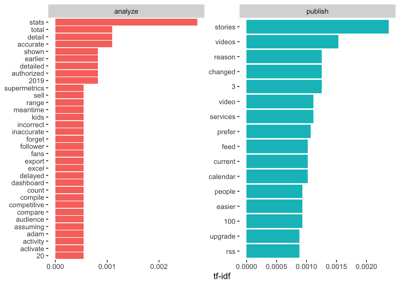
For Analyze, accuracy and details seem to be important reasons for churning. For Publish, stories and videos appear to be important.

We can also consider groups of words as tokens. Bigrams are groups of two words, trigrams are groups of three, and so on.

# get bigrams
bigrams <- users %>%
  unnest_tokens(bigram, details, token = "ngrams", n = 2)

# separate the words
bigrams_separated <- bigrams %>%
  separate(bigram, c("word1", "word2"), sep = " ")

# filter out stop words
bigrams_filtered <- bigrams_separated %>%
  filter(!word1 %in% stop_words$word) %>%
  filter(!word2 %in% stop_words$word) %>% 
  filter(!is.na(word1) & !is.na(word2))

# new bigram counts:
bigram_counts <- bigrams_filtered %>% 
  count(word1, word2, sort = TRUE)

# view top bigrams
head(bigram_counts)

## # A tibble: 6 x 3
##   word1   word2      n
##   <chr>   <chr>  <int>
## 1 social  media    113
## 2 covid   19        63
## 3 free    plan      51
## 4 creator studio    40
## 5 budget  cuts      32
## 6 love    buffer    28

Nice to see “love buffer” in there. Next we’ll visualize the network of bigrams by looking at words that have strong correlations with other words. I’ll spare you a long explanation of the methodology for creating this plot.

library(igraph)
library(ggraph)

# reunite bigrams
bigrams_united <- bigrams_filtered %>%
  unite(bigram, word1, word2, sep = " ")

# filter for only relatively common combinations
bigram_graph <- bigram_counts %>%
  filter(n >= 8) %>%
  graph_from_data_frame()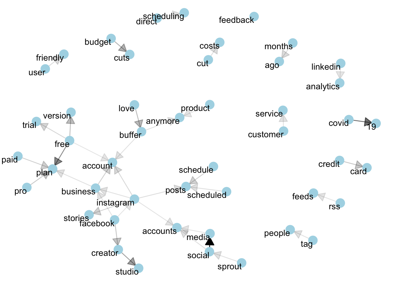

We can see relationships between terms here. Things like covid -> 19 and credit -> card are straightforward. It’s nice to see linkedin -> analytics in this graphs since we just lauched that feature. Instagram seems to be a central node, with many other nodes correlated to it.

Next let’s find the words that are appearing at greater frequencies in our churn survey responses. In order to do this we’ll calculate the relative frequency of each term in each month and fit a linear model to find frequencies that are growing most quickly.

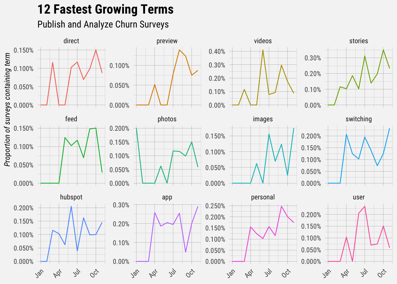
The frequencies of the terms terms “direct”, “preview”, “videos”, and “stories” have grown the most over the past year.

Conclusion

This is a small taste of what’s possible with text analysis. There are rich text datasets to explore and more methods to try.