How "On Time" Are Buffer's Posts?

TLDR: Pretty on-time.

In this analysis we’ll look at how well Buffer does in sending posts out in time. We’ll look at a random sample of 1 million recent Publish updates and compare the sent_at and due_at times.

It’s important to note that we’re excluding failed posts and only looking at updates with a status of “sent”. This excludes Instagram reminders that were sent to mobile devices and all posts with different statuses. We’re also only looking at records in which there are valid sent_at and due_at values.

Conclusions

Approximately 2% of Publish posts sent since February 2021 were sent at least one minute late.
Instagram posts were significantly more likely to be sent late. Around 6% of IG posts were late.
The vast majority of late posts (95%) were only one minute late or less.
Around 90% of posts are sent within 31 seconds of the scheduled time.
Around 95% of posts are sent within 43 seconds of the scheduled time.
Around 98% of posts are sent within 60 seconds of the scheduled time.
Around 99% of posts are sent within 69 seconds of the scheduled time.

How Many Posts Are Delayed?

Let’s calculate the proportion of posts that were sent at least one minute after they were scheduled to post.

# count proportion that were late
posts %>% 
  group_by(late = delay_minutes >= 1) %>% 
  summarise(posts = n_distinct(id)) %>% 
  mutate(percent = scales::percent(posts / sum(posts), accuracy = 0.01))

## # A tibble: 2 x 3
##   late   posts percent
##   <lgl>  <int> <chr>  
## 1 FALSE 979329 97.93% 
## 2 TRUE   20671 2.07%

Around 2% of posts were sent at least one minute after they were due. We can also check if this differs by social network.

## # A tibble: 5 x 4
## # Groups:   service [5]
##   service   late  posts percent
##   <chr>     <lgl> <int> <chr>  
## 1 instagram TRUE   8318 6%     
## 2 facebook  TRUE   6021 2%     
## 3 linkedin  TRUE   1329 1%     
## 4 pinterest TRUE    291 1%     
## 5 twitter   TRUE   4712 1%

Instagram posts were the most likely to be sent out late, with ~6% being sent at least one minute after they were due.

Now we’ll visualize how late the posts were (in minutes).

# define cuts
cuts <- c(-Inf, 0, 1, 5, 10, 60, Inf)

# bucket delays
posts %>% 
  mutate(delay_bucket = cut(delay_minutes, breaks = cuts)) %>% 
  group_by(delay_bucket) %>% 
  summarise(posts = n_distinct(id)) %>% 
  mutate(percent = scales::percent(posts / sum(posts)))

## # A tibble: 6 x 3
##   delay_bucket  posts percent 
##   <fct>         <int> <chr>   
## 1 (-Inf,0]     979329 97.9329%
## 2 (0,1]         19670 1.9670% 
## 3 (1,5]           577 0.0577% 
## 4 (5,10]          373 0.0373% 
## 5 (10,60]          15 0.0015% 
## 6 (60, Inf]        36 0.0036%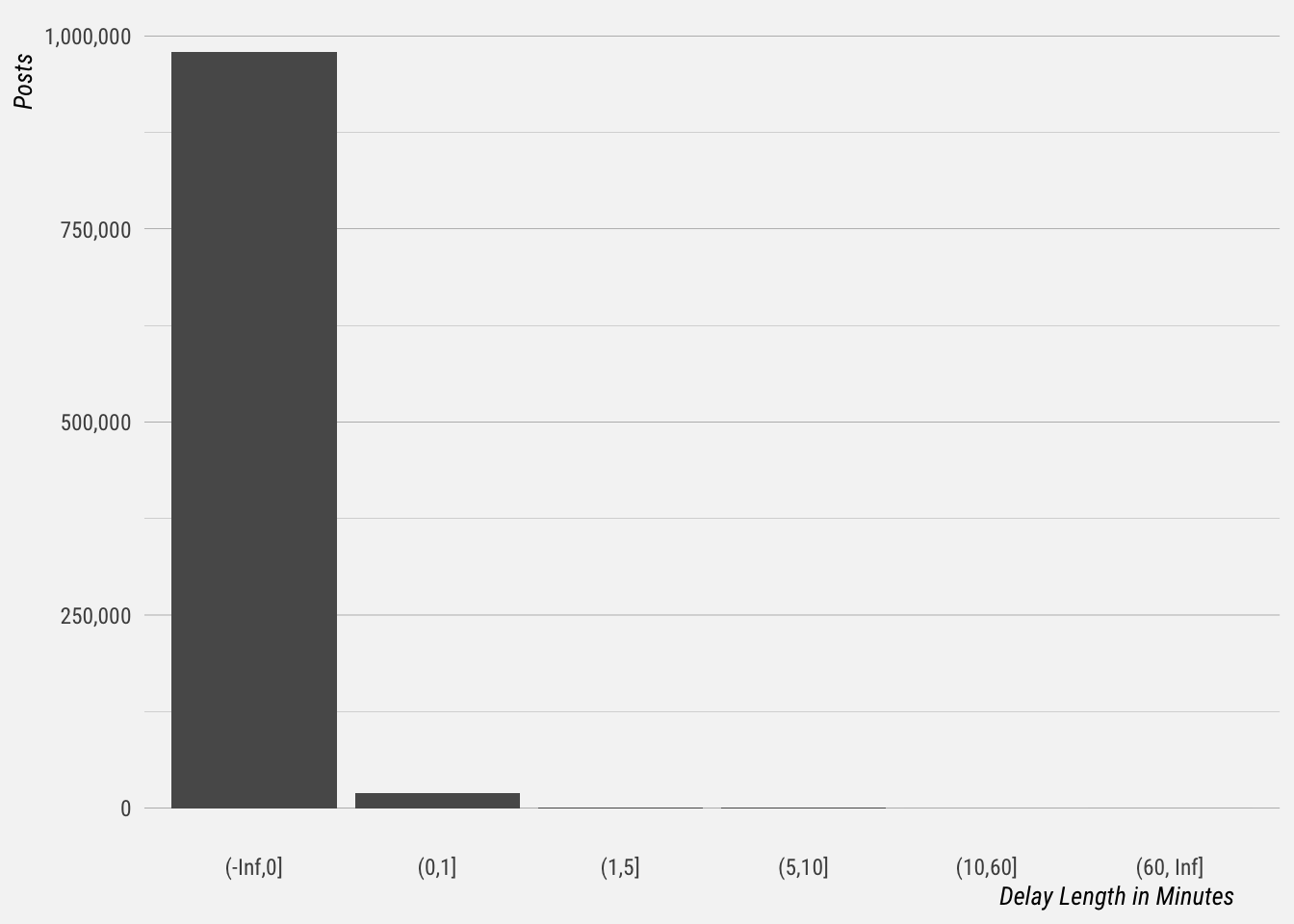

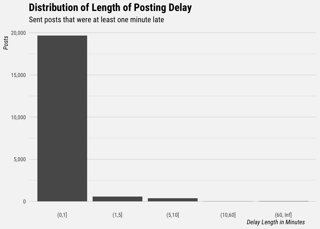
Let’s only look at posts that were at least one minute late.

Now let’s break it down by channel.

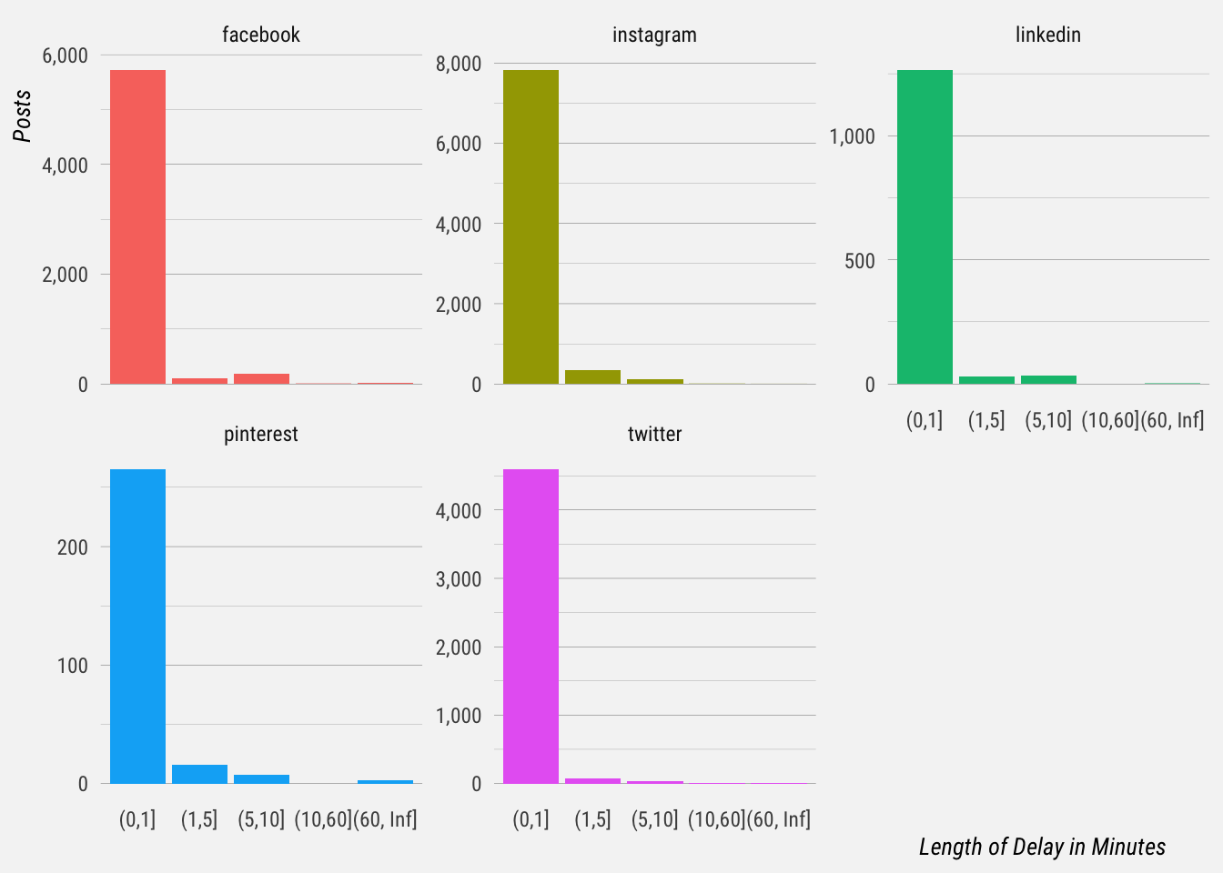
Most delays appear to be only one minute in length, although there are cases in which updates were sent significantly later.

Delay in Seconds

Another way to visualize Buffer’s performance is to plot the cumulative distribution function (CDF).

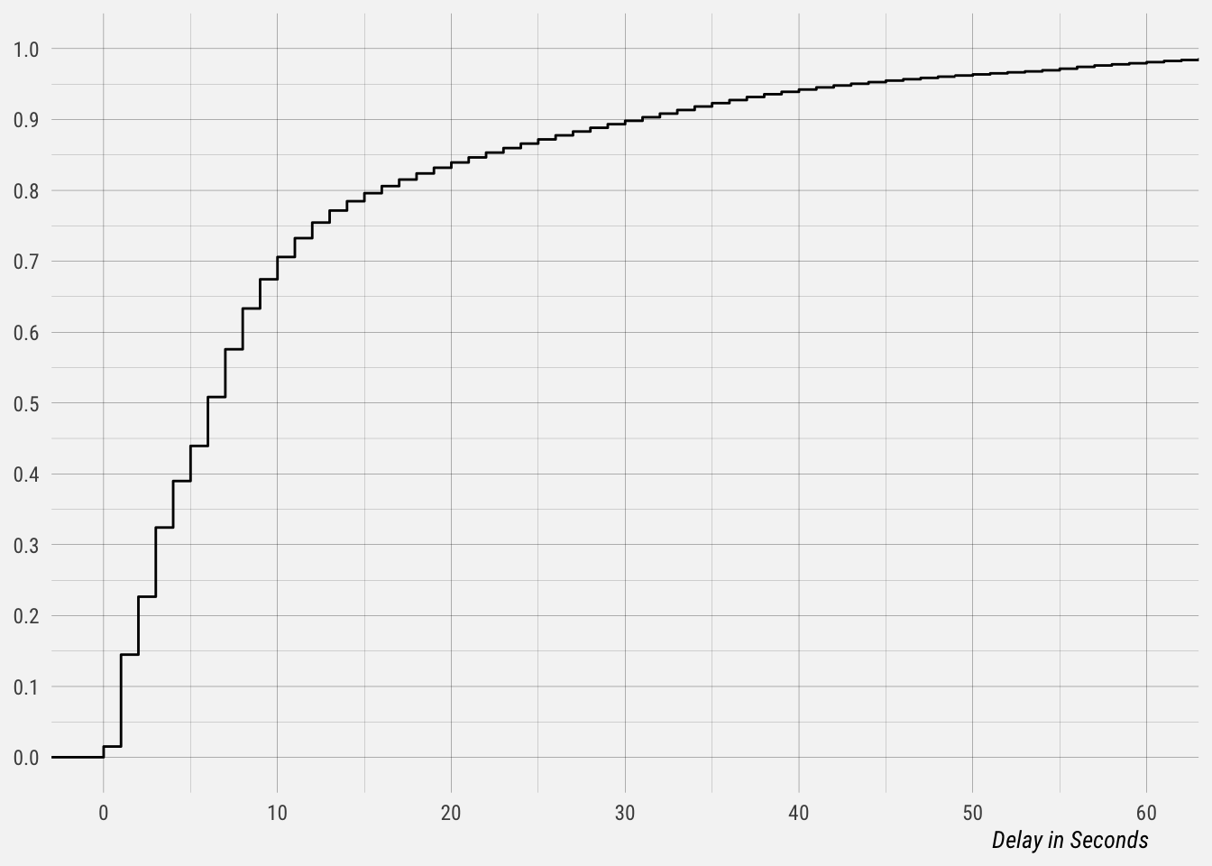
Here’s how I’d interpret this graph:

Around 90% of posts are sent within 31 seconds of the scheduled time.
Around 95% of posts are sent within 43 seconds of the scheduled time.
Around 98% of posts are sent within 60 seconds of the scheduled time.
Around 99% of posts are sent within 69 seconds of the scheduled time.

Here’s how we get the exact values.

# get percentiles
quantile(posts$delay_seconds, probs = c(0.9, 0.95, 0.98, 0.99))

## 90% 95% 98% 99% 
##  31  43  60  69