Text Analysis of NPS Survey Responses

Tidy Text Data Format

In order to analyze the text efficiently, we’ll want to make use of some “tidy” data principles. To consider this data set tidy we need to have one token (or one observation in most other analyses) per row. A token in this text analysis is one word or a group of words.

# unnnest the tokens
text_df <- nps %>%
  unnest_tokens(word, text)

# glimpse data
glimpse(text_df)

## Rows: 25,162
## Columns: 5
## $ date        <date> 2021-04-21, 2021-04-21, 2021-04-21, 2021-04-21, 2021-04-…
## $ user_id     <chr> "5ca1d70e1d99bc38dbf7e439", "5ca1d70e1d99bc38dbf7e439", "…
## $ rating      <int> 0, 0, 0, 0, 0, 0, 0, 0, 1, 1, 1, 1, 1, 1, 1, 1, 1, 1, 1, …
## $ nps_segment <chr> "detractor", "detractor", "detractor", "detractor", "detr…
## $ word        <chr> "do", "not", "disturb", "me", "with", "this", "stupid", "…

Next we’ll remove stop words like “a”, “the”, etc. that aren’t useful to us.

# get stop words
data(stop_words)

# remove stop words from dataset
text_df <- text_df %>%
  anti_join(stop_words, by = "word")

Data Exploration

Now that the data has been restructured into a tidy format, we can do some exploration. Let’s start by looking at the most common terms present in the NPS survey responses.

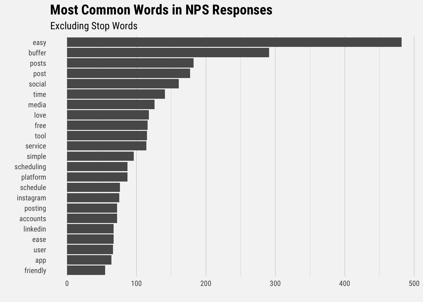
It’s great to see that “easy” is the most common word in our NPS survey responses. It’s easy to see themes of simplicity and saving time. Now let’s look at the top words for each NPS segment.

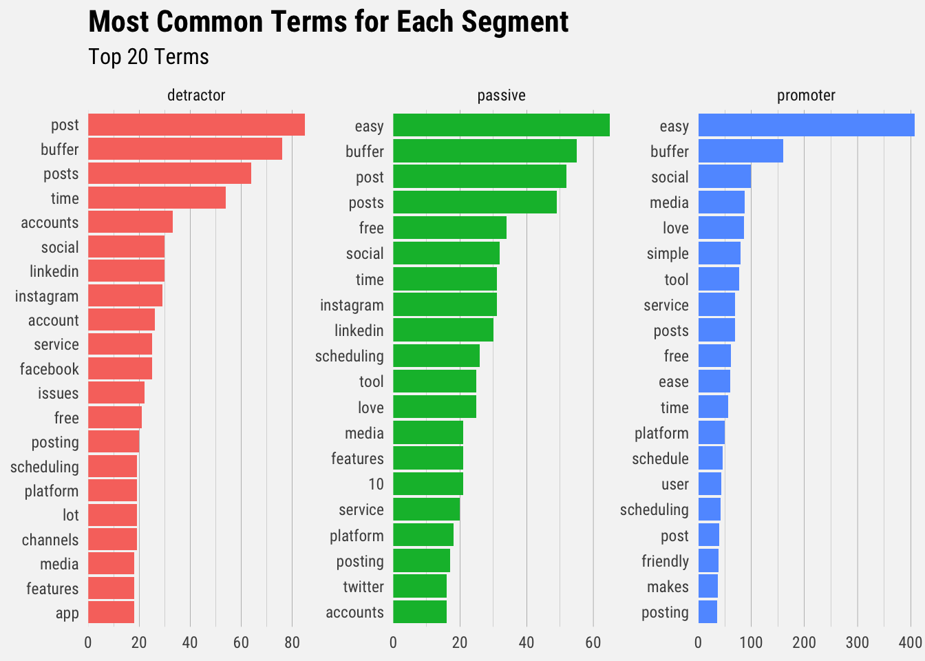
We can see that there are words that appear frequently for all three segments (e.g. “buffer”, “post”). To address this we’ll use a different technique to look at words that occur with more frequency for promoters than for detractors or passives.

To find these words, we can calculate the relative frequency of words that appear in promoters’ responses and compare that to the relative frequency of the words that appear in detractors’.

The idea of term frequency–inverse document frequency (tf-idf) is to find the important words for the content of each document by decreasing the weight for commonly used words and increasing the weight for words that are not used very much in a collection or corpus of documents, in this case, all survey responses for each segment. Calculating tf-idf attempts to find the words that are common in a text document, but not too common.

# get all words in the survey
survey_words <- nps %>%
  unnest_tokens(word, text) %>%
  anti_join(stop_words, by = "word") %>% 
  count(nps_segment, word, sort = TRUE)

# get total of all words
total_words <- survey_words %>% 
  group_by(nps_segment) %>% 
  summarize(total = sum(n))

# join to get proportions
survey_words <- left_join(survey_words, total_words)
head(survey_words) 

## # A tibble: 6 x 4
##   nps_segment word       n total
##   <chr>       <chr>  <int> <int>
## 1 promoter    easy     408  4433
## 2 promoter    buffer   160  4433
## 3 promoter    social    99  4433
## 4 promoter    media     87  4433
## 5 promoter    love      86  4433
## 6 detractor   post      85  3148

The bind_tf_idf() function takes a tidy text data set as input with one row per token, per document. One column (word) contains the tokens, one column contains the documents (nps_segment), and the last necessary column contains the counts, how many times each document contains each term (n).

# calculate tf-idf
segment_tf_idf <- survey_words %>%
  bind_tf_idf(word, nps_segment, n)

The idf term is very low for words that appear frequently for each segment. The inverse document frequency (and thus tf-idf) is very low (near zero) for words that occur in many of the documents in a collection; this is how this approach decreases the weight for common words. The inverse document frequency will be a higher number for words that occur in fewer of the documents in the collection.

Let’s look at words with high tf-idf in the NPS surveys.

# high tf-idf words
segment_tf_idf %>%
  select(-total) %>%
  arrange(desc(tf_idf)) %>% 
  head()

## # A tibble: 6 x 6
##   nps_segment word          n      tf   idf  tf_idf
##   <chr>       <chr>     <int>   <dbl> <dbl>   <dbl>
## 1 promoter    excellent    29 0.00654  1.10 0.00719
## 2 promoter    amazing      17 0.00383  1.10 0.00421
## 3 promoter    fantastic    11 0.00248  1.10 0.00273
## 4 detractor   bad           7 0.00222  1.10 0.00244
## 5 detractor   clunky        7 0.00222  1.10 0.00244
## 6 promoter    layout        9 0.00203  1.10 0.00223

This checks out. The terms “excellent”, “amazing”, and “fantastic” appear relatively frequently in Promoters’ responses, whereas the terms “bad”, “clunky”, and “layout” appear relatively frequently for detractors.

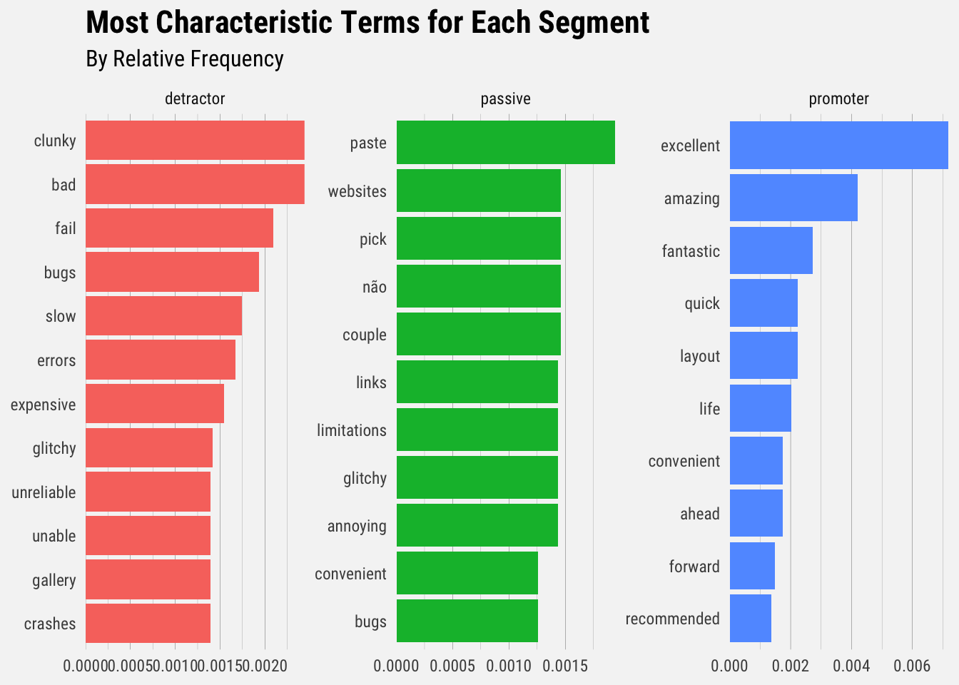
We can start to pick up themes that appear for detractors and promoters. Detractors mention poor performance and reliability, whereas promoters do not. Passives seem to resemble detractors more than promoters.

Bigrams

We can also consider groups of words as tokens. Bigrams are groups of two words, trigrams are groups of three, and so on.

# get bigrams
bigrams <- nps %>%
  unnest_tokens(bigram, text, token = "ngrams", n = 2)

# separate the words
bigrams_separated <- bigrams %>%
  separate(bigram, c("word1", "word2"), sep = " ")

# filter out stop words
bigrams_filtered <- bigrams_separated %>%
  filter(!word1 %in% stop_words$word) %>%
  filter(!word2 %in% stop_words$word) %>% 
  filter(!is.na(word1) & !is.na(word2))

# new bigram counts:
bigram_counts <- bigrams_filtered %>% 
  count(word1, word2, sort = TRUE)

# view top bigrams
head(bigram_counts, 10)

## # A tibble: 10 x 3
##    word1    word2         n
##    <chr>    <chr>     <int>
##  1 social   media       122
##  2 user     friendly     47
##  3 free     version      25
##  4 customer service      18
##  5 media    posts        16
##  6 super    easy         16
##  7 love     buffer       15
##  8 media    accounts     15
##  9 tag      people       15
## 10 multiple platforms    13

It’s great to see bigrams like “super easy” and “user friendly”. Next we’ll visualize the network of bigrams by looking at words that have strong correlations with other words. I’ll spare you a long explanation of the methodology for creating this plot.

library(igraph)
library(ggraph)

# reunite bigrams
bigrams_united <- bigrams_filtered %>%
  unite(bigram, word1, word2, sep = " ")

# filter for only relatively common combinations
bigram_graph <- bigram_counts %>%
  filter(n >= 4) %>%
  graph_from_data_frame()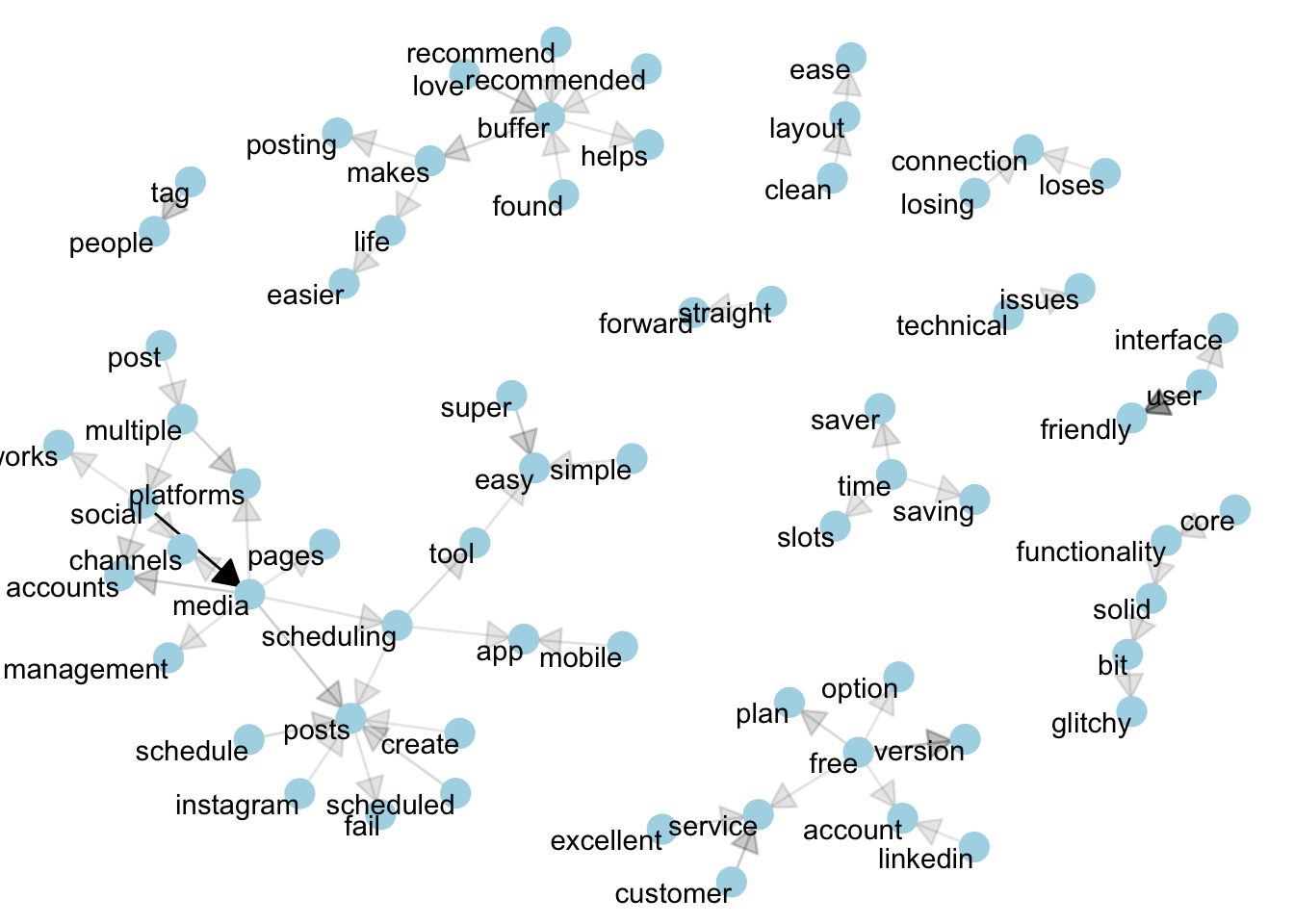

Here we can see the relationships between terms. Things like people -> tag and technical -> issues make sense. “Posts” and “media” appear to be central nodes, as well as “loses/losing connection”.

Let’s recreate this plot only for detractors and passives.

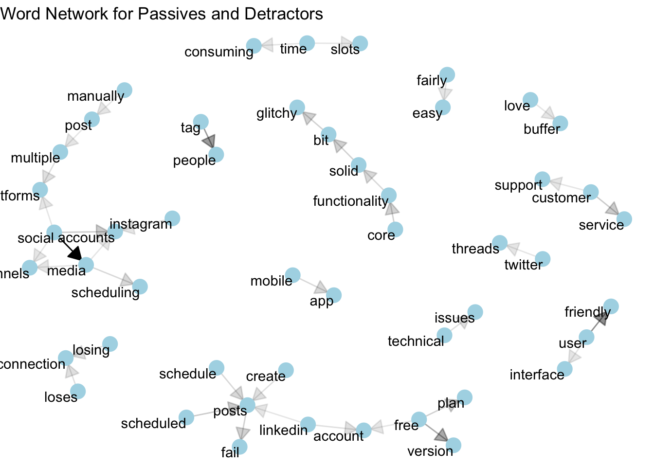
These are the related terms for detractors and passives. Core functionality, technical issues, losing connection, people tagging, and time consuming slots are all interesting things to potentially look into. It’s nice to see that “love buffer” is still present.

Topic Modeling

# load library
library(topicmodels)

## Warning: package 'topicmodels' was built under R version 3.6.2

library(tm)

## Warning: package 'tm' was built under R version 3.6.2

# cast to document term matrix
desc_dtm <- top_terms %>%
  cast_dtm(nps_segment, word, n)

# create LDA model
desc_lda <- LDA(desc_dtm, k = 2, control = list(seed = 1234))
desc_lda

## A LDA_VEM topic model with 2 topics.

# tidy results of model
tidy_lda <- tidy(desc_lda)

# get top terms per topic
top_terms <- tidy_lda %>%
  group_by(topic) %>%
  slice_max(beta, n = 10, with_ties = FALSE) %>%
  ungroup() %>%
  arrange(topic, -beta)

# plot
top_terms %>%
  mutate(term = reorder_within(term, beta, topic)) %>%
  group_by(topic, term) %>%    
  arrange(desc(beta)) %>%  
  ungroup() %>%
  ggplot(aes(beta, term, fill = as.factor(topic))) +
  geom_col(show.legend = FALSE) +
  scale_y_reordered() +
  labs(title = "Top 10 terms in each LDA topic",
       x = expression(beta), y = NULL) +
  facet_wrap(~ topic, ncol = 2, scales = "free")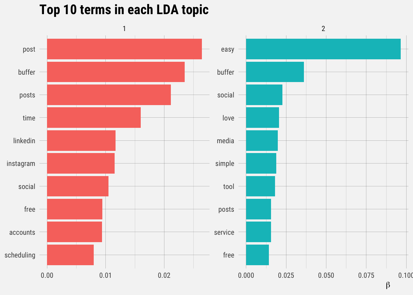

What’s Next

Once some time is pass, we can do some more analysis to see which terms are appearing more or less frequently over time.