Distribution of Profiles for Paying Publish Users

Data Tidying

Let’s determine if each profile is active, and then count active and inactive profiles for each user.

# determine if active
profiles <- profiles %>% 
  mutate(is_active = updates >= 1,
         dollar_amount = plan_amount / 100)

# group by user
by_user <- profiles %>% 
  group_by(user_id, billing_plan, plan_id, quantity, customer_id,
           product, dollar_amount, billing_interval, is_active) %>% 
  summarise(profiles = n_distinct(profile_id)) %>% 
  pivot_wider(names_from = is_active, 
              values_from = profiles) %>% 
  replace_na(list(`TRUE` = 0, `FALSE` = 0))

## `summarise()` regrouping output by 'user_id', 'billing_plan', 'plan_id', 'quantity', 'customer_id', 'product', 'dollar_amount', 'billing_interval' (override with `.groups` argument)

# rename columns
names(by_user) <- c("user_id", "billing_plan", "plan_id", "quantity", "customer_id",
                    "product", "dollar_amount", "billing_interval",
                    "inactive_profiles", "active_profiles")

# get total profiles
by_user <- by_user %>% 
  mutate(total_profiles = inactive_profiles + active_profiles)

# see how many users are on each plan
by_user %>% 
  ungroup %>% 
  filter(billing_plan != "individual" & billing_plan != "awesome") %>% 
  count(billing_plan, sort = T)

## # A tibble: 10 x 2
##    billing_plan      n
##    <chr>         <int>
##  1 pro           51560
##  2 small          7258
##  3 premium        3830
##  4 premium_v2     1588
##  5 business        624
##  6 agency          201
##  7 enterprise       15
##  8 enterprise150     8
##  9 enterprise200     4
## 10 enterprise300     3

We’ll group the enterprise plans together before plotting the distributions.

# group enterprise plans
by_user <- by_user %>% 
  filter(billing_plan != "individual" & billing_plan != "awesome") %>% 
  mutate(billing_plan = gsub("enterprise150", "enterprise", billing_plan)) %>% 
  mutate(billing_plan = gsub("enterprise200", "enterprise", billing_plan)) %>% 
  mutate(billing_plan = gsub("enterprise300", "enterprise", billing_plan))

Distribution of Profiles

We’ll start by plotting histograms of the total number of profiles connected for users on each plan type.

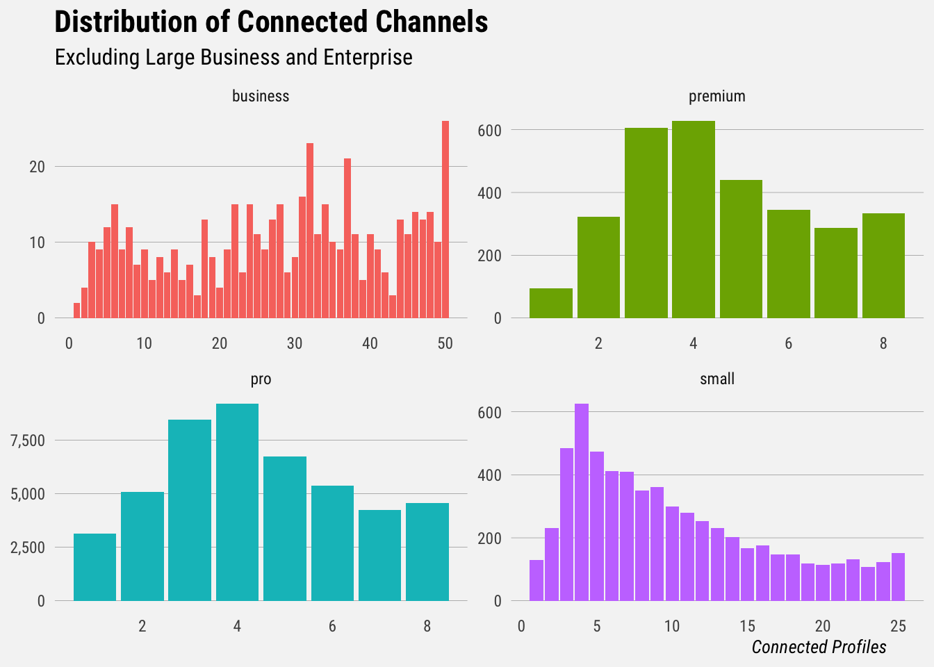
We’ll export a csv of counts for each plan for internal use.

by_user %>% 
  group_by(billing_plan, total_profiles) %>% 
  summarise(users = n_distinct(user_id)) %>% 
  ungroup %>% 
  filter(
    case_when(
      billing_plan == "pro" ~ total_profiles <= 8,
      billing_plan == "small" ~ total_profiles <= 25,
      billing_plan == "business" ~ total_profiles <= 50,
      billing_plan == "premium" ~ total_profiles <= 8,
      TRUE ~ total_profiles <= 1000
    )
  ) %>% 
  write.csv(file = "~/Desktop/all_connected_profile_counts.csv", row.names = F)

Next we’ll plot the distributions of active profiles.

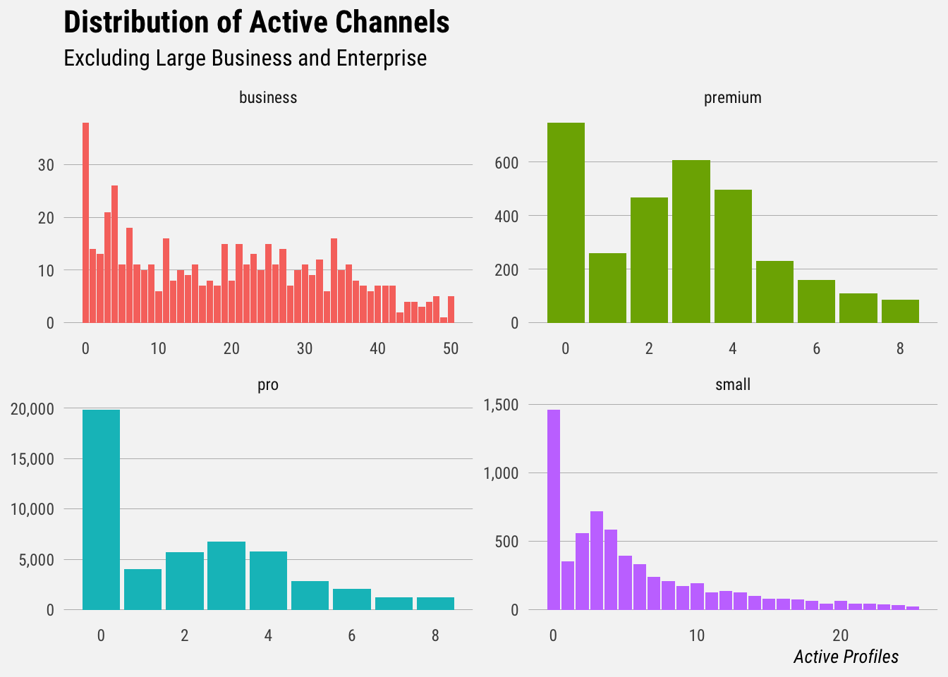
We can export another csv of counts for each plan.

by_user %>% 
  group_by(billing_plan, active_profiles) %>% 
  summarise(users = n_distinct(user_id)) %>% 
  ungroup %>% 
  filter(
    case_when(
      billing_plan == "pro" ~ active_profiles <= 8,
      billing_plan == "small" ~ active_profiles <= 25,
      billing_plan == "business" ~ active_profiles <= 50,
      billing_plan == "premium" ~ active_profiles <= 8,
      TRUE ~ active_profiles <= 1000
    )
  ) %>% 
  write.csv(file = "~/Desktop/active_profile_counts.csv", row.names = F)