Analysis of New Buffer Subscription Churn

Summary of Findings

So far, New Buffer subscriptions appear to be churning at lower rates than Publish subscriptions created since the beginning of 2020. This difference is statistically significant.

Because New Buffer subscriptions haven’t yet dropped to 50% survival – there have only been approximately 263 churn events from 3103 New Buffer subscriptions – the differences in median survival time can’t yet be calculated. We’ll have to circle back to that in a couple months.

Data Collection

The data we’ll use in this analysis consists of around 58 thousand subscriptions started since the beginning of 2020. Of these around 3 thousand are New Buffer subscriptions.

There are a couple important things to note. We’re only including Stripe subscriptions in this analysis, so the subscription churn rates of mobile subscriptions are not included.

I’ve also come across several subscriptions created by members of the Buffer team, presumably when testing. These subscriptions appear to have churned very quickly, so it’s possible that they may influence churn rates.

I also want to mention that the current plan ID is used to determine whether a subscription is a New Buffer subscription. If an old subscription that started on an Awesome plan was upgraded to a New Buffer plan at a certain point, the subscription is considered to be New Buffer and the length of the subscription, including the time on an Awesome plan, is used in the analysis.

Data Tidying

There are a few things we need to do to the data before it’s ready for analysis. We’ll want to exclude subscriptions that are trialing or in a past-due state. We’ll also set a new variable, surv_status, that indicates whether a subscription has been canceled.

We’ll also calculate the number of days that it took the subscription to cancel. If the data is censored, i.e. the subscription is still active, we calculate the number of days that have elapsed since the subscription was started.

# gather data
subs <- readRDS("ob_sub_retention.rds")

# determine if sub is canceled
subs <- subs %>% 
  filter(status == "canceled" | status == "active") %>% 
  filter(is.na(product) | product == "publish") %>% 
  mutate(canceled = status == "canceled",
         surv_status = ifelse(canceled, 1, 0)) %>% 
  replace_na(list(end_date = Sys.Date())) %>% 
  mutate(time_to_cancel = as.numeric(end_date - start_date)) %>% 
  filter(time_to_cancel >= 0)

Below is a glimpse of the survival data. The numbers indicates the number of days to either a cancellation event or censoring. The data that is censored has a “+” after the number, indicating that the time to churn is at least X days.

# build survival object
km <- Surv(subs$time_to_cancel, subs$canceled)

# preview data
head(km, 10)

##  [1]  76   81   31  576+ 107+ 618+ 102   50   97+   3

Next we want to determine if the subscriptions are New Buffer subscriptions. We’ll look at the plan IDs to do this.

# one buffer plans
ob_plans <- c("buffer_essentials_m_5_202104", "buffer_essentials-team_m_10_202104",
             "buffer_essentials_y_48_202104", "buffer_essentials-team_y_96_202104",
             "buffer_essentials_y_60_202106", "buffer_essentials_m_6_202106",
             "buffer_essentials-team_y_120_202106",
             "buffer_essentials-team_m_12_202106")

# monthly ob plans
monthly_ob_plans <- c("buffer_essentials_m_5_202104",
                      "buffer_essentials-team_m_10_202104",
                      "buffer_essentials_m_6_202106",
                      "buffer_essentials-team_m_12_202106")

# indicator of one buffer
subs <- subs %>% 
  mutate(is_ob = plan_id %in% ob_plans,
         is_ob_monthly = plan_id %in% monthly_ob_plans)

Survival Analysis

Now we’re ready for the survival analysis. We’ll estimate the survival curve for the entire dataset with the Kaplan-Meier method. This curve shows the estimated probability of surviving X days for all of the subscriptions in the dataset.

# create kaplan-meier survival curve
fit.surv <- survfit(Surv(time_to_cancel, surv_status) ~ 1, data = subs)

# plot survival curve
autoplot(fit.surv, censor = TRUE, censor.size = 1) +
  scale_x_continuous(limits = c(0, 365)) +
  scale_y_continuous(limits = c(0.4, 1), labels = percent) +
  labs(x = "Days", y = "Estimated Probability of Survival",
       title = "Survival Curve of Buffer Stripe Subscriptions",
       subtitle = "All Publish and New Buffer Subscriptiosn Created Since 2020")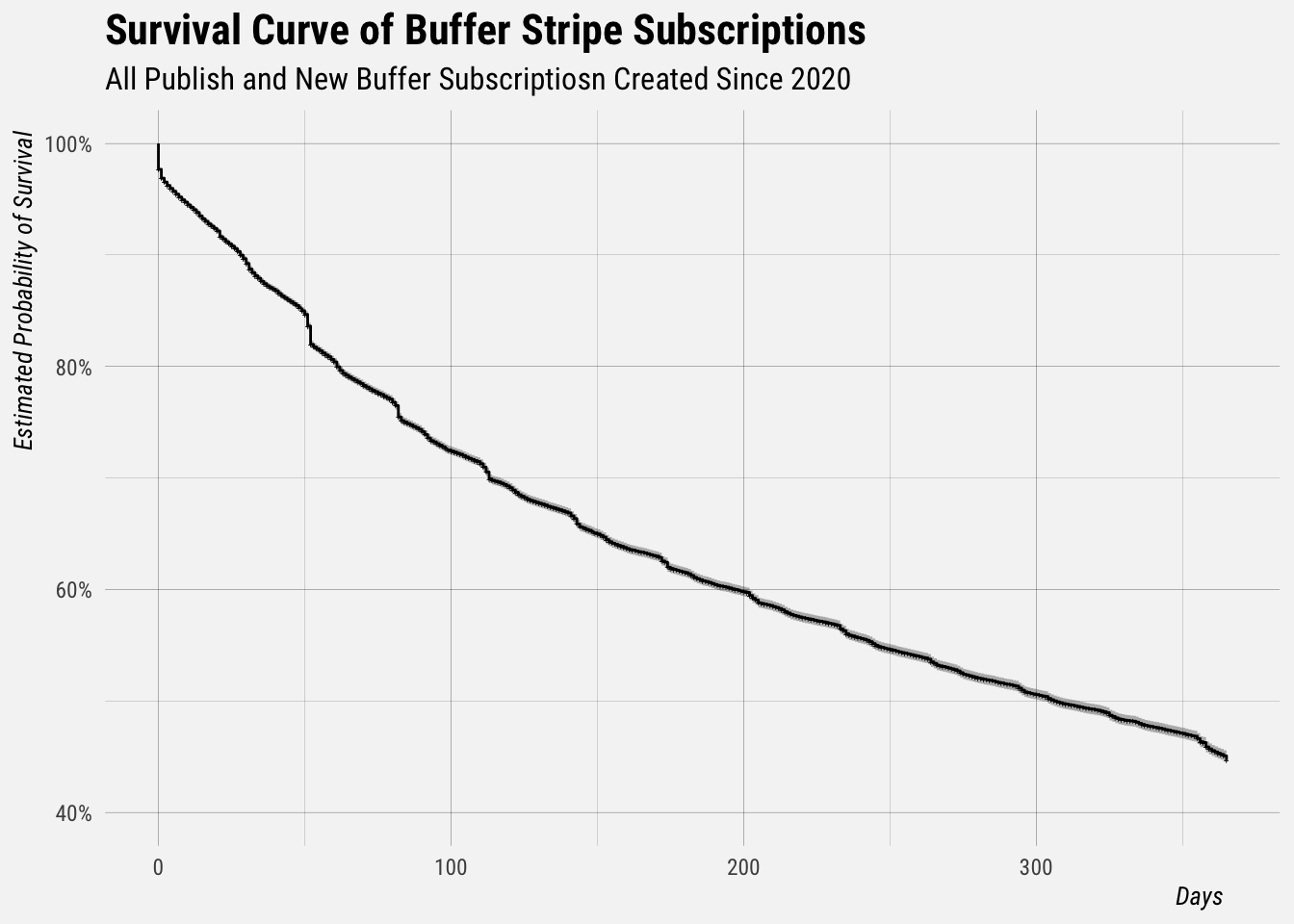

Next we’ll stratify the survival curve using the is_ob label to compare the survival probabilities of Publish and New Buffer subscriptions.

# create survival curves stratified by whether plans are New Buffer
fit.ob <- survfit(Surv(time_to_cancel, surv_status) ~ is_ob, data = subs)

# plot stratified curves
autoplot(fit.ob, censor = TRUE, censor.size = 1) +
  scale_x_continuous(limits = c(0, 180)) +
  scale_y_continuous(limits = c(0.6, 1), labels = percent) +
  labs(x = "Days", y = "Estimated Probability of Survival",
       title = "Survival Curves of Stripe Subscriptions",
       subtitle = "All Publish and New Buffer Subscriptiosn Created Since 2020") +
  scale_color_discrete(name = "New Buffer") +
  scale_fill_discrete(name = "New Buffer")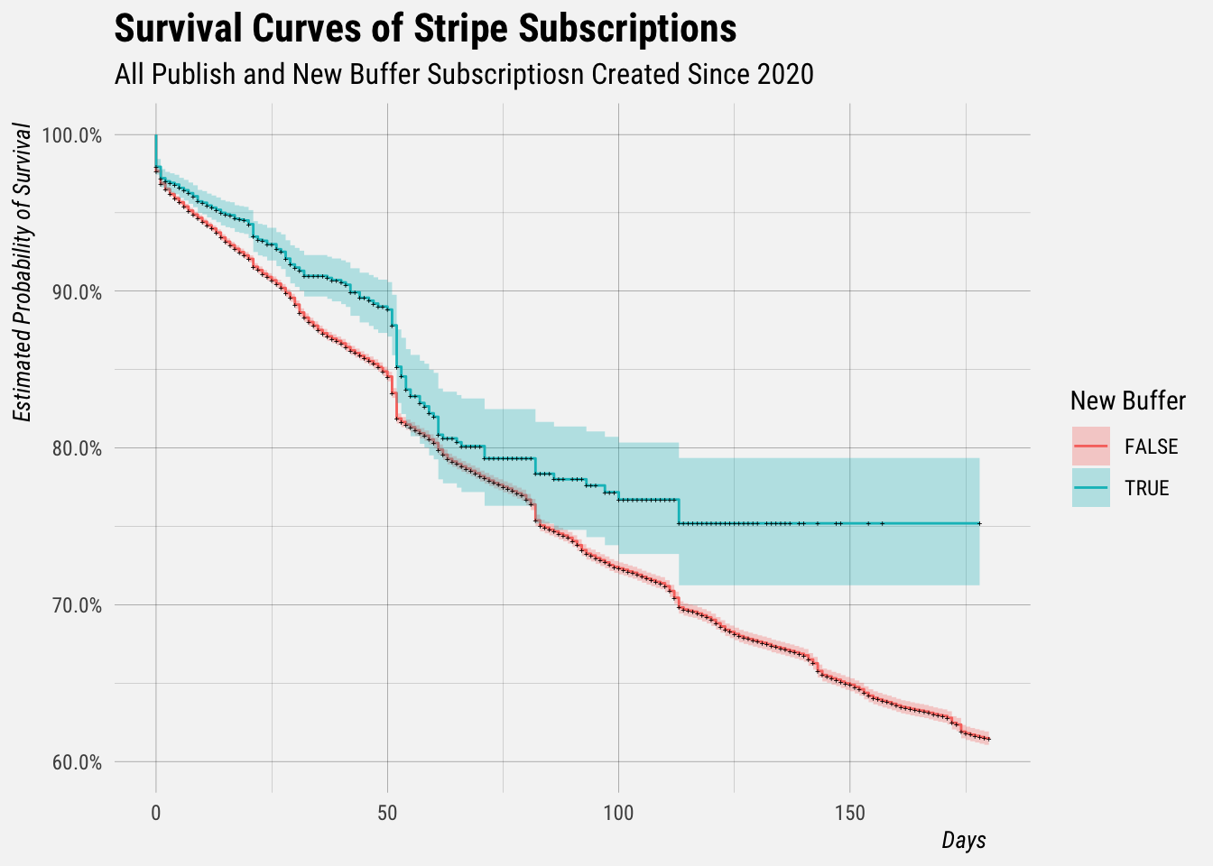

We can see that the survival curve of New Buffer subscriptions is higher than that of Publish subscriptions, which suggests that the churn rates are lower.

There is a formal way to test if whether the survival distributions are truly different, the Log-Rank Test.

Log-Rank Test

The log-rank test is a hypothesis test to compare the survival distributions of two samples. It’s a nonparametric test and appropriate to use when the data are right skewed and censored. It is widely used in clinical trials to establish the efficacy of a new treatment in comparison with a control treatment when the measurement is the time to event (such as the time from initial treatment to a heart attack).

For us it’s a useful way to tell if the survival curve of New Buffer subscriptions is significantly different to that of Publish subscriptions.

# perform log-rank test
logrank.test <- survdiff(Surv(time_to_cancel, surv_status) ~ is_ob, data = subs)
logrank.test

## Call:
## survdiff(formula = Surv(time_to_cancel, surv_status) ~ is_ob, 
##     data = subs)
## 
##                 N Observed Expected (O-E)^2/E (O-E)^2/V
## is_ob=FALSE 54990    27668    27587     0.235      19.7
## is_ob=TRUE   3103      263      344    18.899      19.7
## 
##  Chisq= 19.7  on 1 degrees of freedom, p= 9e-06

The low p-value of this test (0.0002) tells us that there is a statistically significant difference in the two survival distributions.

Cox Proportional Hazard Models

Next we’ll fit a Cox model to estimate the effect that New Buffer has on subscription churn given other predictors. In this case, we’ll look at the effect of New Buffer given the plan interval, i.e. whether it was billed monthly or annually.

We’ve seen in another analysis that New Buffer customers are more likely to choose annual plans, which tend to have lower churn rates. This model will help us compare New Buffer monthly plans to monthly Publish subscriptions.

# fit cox model
fit.cox <- coxph(Surv(time_to_cancel, surv_status) ~ is_ob + interval, data = subs)
fit.cox

## Call:
## coxph(formula = Surv(time_to_cancel, surv_status) ~ is_ob + interval, 
##     data = subs)
## 
##                  coef exp(coef) se(coef)       z        p
## is_obTRUE    -0.25147   0.77765  0.06247  -4.026 5.69e-05
## intervalyear -1.38837   0.24948  0.01751 -79.303  < 2e-16
## 
## Likelihood ratio test=8521  on 2 df, p=< 2.2e-16
## n= 58092, number of events= 27930 
##    (1 observation deleted due to missingness)

The negative coefficients of the model indicate a positive effect on the survival of the subscriptions. The results indicate that the risk of churn for annual subscriptions is around four times (i.e. e^1.39 = 4) less than that of monthly subscriptions. The risk of churn for New Buffer subscriptions is around 29% (e^0.25 = 1.29) less than that of Publish subscriptions.

In other words, after adjusting for the plan interval, New Buffer subscribers are significantly less likely to cancel than Publish subscribers.

Median Survival Time

We can also use the median survival time to estimate the difference in survival distributions. However, since the sample of New Buffer subscriptions hasn’t yet dropped to 50% survival (only 263 churn events from 3103 subscriptions), the median can’t yet be calculated. We’ll have to try this again later.

# summarise survival 
survfit(Surv(time_to_cancel, surv_status) ~ is_ob, data = subs)

## Call: survfit(formula = Surv(time_to_cancel, surv_status) ~ is_ob, 
##     data = subs)
## 
##                 n events median 0.95LCL 0.95UCL
## is_ob=FALSE 54990  27668    306     301     313
## is_ob=TRUE   3103    263     NA      NA      NA